Variation
Variation describes how one variable changes in relation to another. In direct variation, as one variable increases, the other increases proportionally. In inverse variation, one variable decreases proportionally as the other increases. These variations form the basis of mathematical formulas that connect variables and support data transformations, even in cases involving non-linear relationships. Understanding both direct and inverse variation is essential in fields like physics, economics, and engineering, where analysing the relationship between variables is important for accurate predictions and decision-making.
Use this page to revise the following concepts of variation:
Direct Variation
In direct variation, two variables \(x\) and \(y\) are related by the equation \(y = kx\), where \(k\) is a positive constant. As \(x\) increases, \(y\) increases. This relationship is described as ‘\(y\) varies directly as \(x\)’ or '\(y\) is directly proportional to \(x\)’, and can be written symbolically as \(y \propto x\).
The constant \(k\) is known as the constant of variation, and is calculated using the formula:
\[k = \frac{\text{y value}}{\text{corresponding to the value of x}}\]
This means that for any two non-zero values \(x_1\) and \(x_2\), with the corresponding \(y_1\) and \(y_2\), the ratio remains constant:
\[\frac{y_1}{x_1} = \frac{y_2}{x_2} = k\]
For example, if \(y = 5x\), then \(y \propto x\) , and the constant of variation is 5.
The graph of \(y\) against \(x\) is a straight line, passing through the origin. The slope of the line is the constant of variation \(k\).
Note that whilst in all direct variation, as one variable increases, the other also increases, not all increasing trends indicate direct variation.
Example of Direct Variation
An example of direct variation is with the variables \(\text{work done}\) and \(\text{time}\) when working at a constant rate.
For instance, Mark is painting a fence and works at a constant rate, painting 4 metres of the fence every hour. He keeps track of the time and the total length of the fence painted.
| Time (\(t\) hours) | 1 | 2 | 3 | 4 | 5 | 6 |
|---|---|---|---|---|---|---|
| Work done (\(w\) metres) | 4 | 8 | 12 | 16 | 20 | 24 |
It can be seen that, as t increases, w also increases. The rule relating to time and work done is \(w = 4t\). The work done varies directly as the time taken, or, \(w\) is proportional to \(t,\ (w \propto t)\) , where \(4\) is the constant of variation.
As shown below, the graph of \(w\) against \(t\) is a straight line passing through the origin.

Worked Example
The cost (\(C\) in dollars) of tomatoes varies directly with their weight (\(W\) in kilograms).
- If the cost of 3 kg of tomatoes is $9, what is the cost for 5 kg of tomatoes?
- What is the weight of tomatoes if the cost is $36?
Part 1
From the question, we know that \(C \propto W\), therefore \(C = kW\)
When \(W = 3, C = 9\):
\[\begin{align}9 &= k\left(3\right) \\ k&= \frac{9}{3} \\ k &= 3\end{align}\]
The cost for \(5\text{ kg}\) of tomatoes:
\[\begin{align}C &= 3W \\ &= 3\ \times\ 5 \\ &= 15\end{align}\]
The cost for \(5\text{ kg}\) of tomatoes is \(\$15\).
Part 2
\[\begin{align}C &= 3W \\ 36 &= 3W \\ W &= \frac{36}{3} \\ &=12\end{align}\]
If the cost is \(\$36\), the weight of tomatoes is \(12\text{ kg}\).
 Check your understanding
View
Check your understanding
View

Variation involving Powers
In some cases, one of the variables may be raised to a power. For example, if \(y \propto x^n\), then the relationship between the variables \(x\) and \(y\) can be expressed as \(y = kx^n\), where k is a constant of variation. Similarly, the graph of \(y\) against \(x^n\) is a straight line passing through the origin.
Example of Variation involving Powers
For example, a rock is dropped from a cliff, and the distance it falls, in metres, is recorded every second.
| Time (\(t\) seconds) | 0 | 1 | 2 | 3 | 4 | 5 |
|---|---|---|---|---|---|---|
| Distance (\(d\) metres) | 0 | 2.5 | 10 | 22.5 | 40 | 62.5 |
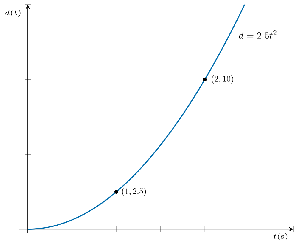
It can be seen that, as \(t\) increases, \(d\) also increases. The rule relating to time and distance is \(d = 2.5 t^2\). In this case, the distance varies directly as the square of the time taken or \(d\) is proportional to \(t^2, \ (w \propto t^2)\) , where \(2.5\) is the constant of variation.
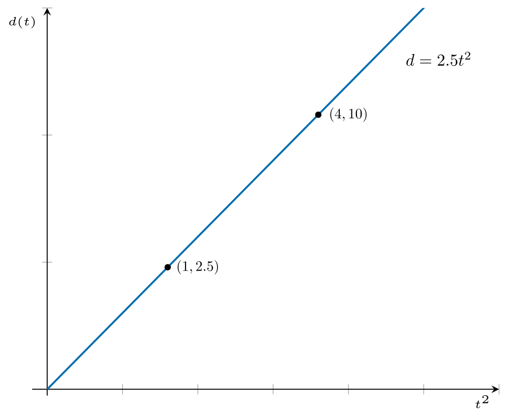
The graph of \(d\) against \(t\) is a parabola, but the graph \(d\) against \(t^{2}\) is a straight line passing through the origin, with a slope of 2.5.
Worked Example
If \(A \propto l^{2}\), and \(A = 72\) when \(l = 6\), find:
- \(A\) when \(l = 5\)
\(l\) when \(A = 100\), correct to one decimal place.
Part 1
From the question, we know that \(A \propto l^{2}, A = k\ \times\ l\)
When \(l = 6, A = 72\):
\[\begin{align}72 &= k\ \times\ 6^{2} \\ 72 &= 36k \\ k &= \frac{72}{36} \\ &=2\end{align}\]
When \(l = 5\):
\[\begin{align}A = 2\ \times\ 5^{2} \\ &= 50\end{align}\]
Part 2
When \(A = 100\):
\[\begin{align}100 &= 2\ \times\ l^{2} \\ l^{2} &= \frac{100}{2} \\ l^{2} &= 50 \\ l &= 7.1\end{align}\]
Check your understanding
View
Inverse Variation
In inverse variation, two variables \(x\) and \(y\) are related by the equation \(y =\frac{k}{x}\), where \(k\) is a positive constant. As \(x\) increases, \(y\) decreases. This relationship is described as ‘\(y\) varies inversely as \(x\)’ or '\(y\) is inversely proportional to \(x\)’, and can be written symbolically as
\[y \propto \frac{1}{x}\]
The constant variation, \(k\), is calculated using the formula:
\[k = xy\]
This means that for any two values \(x_1\) and \(x_2\), with the corresponding \(y_1\) and \(y_2\), the product remains the same:
\[x_1y_1 = x_2y_2 = k\]
This is often a useful method of identifying inverse variation when data is presented in table format.
For example, if \(y = \frac{6}{x}\), then \(y \propto \frac{1}{x}\) , and the constant of variation is \(6\).
The graph of \(y\) against \(x\) forms a curve called a hyperbola. However, the graph of \(y\) against \(\frac{1}{x}\) is a straight line, which excludes a value at the origin (because \(\frac{1}{0}\) is undefined).
Note that in inverse variation, as one variable increases, the other decreases, resulting a decreasing trend on the graph of \(y\) against \(x\). However, not all decreasing trends represent inverse variation.
Example of Inverse Variation
An example of inverse variation is with the variables \(\text{the number of friends}\) and \(\text{cost per person}\).
A group of friends shares the cost of a meal. If two friends split the bill, each pays $6. However, if four friends share the cost, each only pays $3.
| The number of friends (\(n\)) | 1 | 2 | 3 | 4 | 5 | 6 |
|---|---|---|---|---|---|---|
| Cost per person (\(c\) in dollars) | 12 | 6 | 4 | 3 | 2.4 | 2 |
As the number of friends (\(n\)) increases, the cost per person (\(c\) in dollars) decreases. This is an example of inverse variation.
It can be observed that as \(n\) increases, \(c\) decreases. The rule relating to the number of friends and the cost per person is given by the equation \(c = \frac{12}{n}\). The cost per person varies inversely as the number of friends, or \(c\) is proportional to \(\frac{1}{n}\ \left(c \propto \frac{1}{n}\right)\), where \(12\) is the constant variation.
The graph of \(c\) against \(n\) forms a hyperbola.

However, the graph of \(c\) against \(\frac{1}{n}\) is a straight line that does not include the origin.

Worked Example
For a rectangular water tank of fixed volume, the height \((h\text{ cm})\) is inversely proportional to the base length \((l\text{ cm})\).
If a tank with a height of \(12\text{ cm}\) has a base length of \(3\text{ cm}\),
- how high would a tank of equivalent volume be if its base length was \(4.5\text{ cm}\)?
- what would the base length be if the height of the tank was \(10\text{ cm}\)?
Part 1
From the question, we know that \(h \propto \frac{1}{l}, h = \frac{k}{l}\)
The height was \(12\text{ cm}\) when the base length was \(3\text{ cm}\):
\[\begin{align}12 &= \frac{k}{3} \\ k &= 3\ \times\ 12 \\ k &= 36\end{align}\]
The height of the tank when the base length was \(4.5\text{ cm}\):
\[\begin{align}h &= \frac{36}{l} \\ h &= \frac{36}{4.5} \\ h &= 8\end{align}\]
Therefore, a rectangular water tank with a base length of \(4.5\text{ cm}\) has a height of \(8\text{ cm}\).
Part 2
The base length if the height of the tank was \(10\text{ cm}\):
\[\begin{align}h &= \frac{36}{l} \\ 10 &= \frac{26}{l} \\ l &= \frac{36}{10} \\ l &= 3.6\end{align}\]
Therefore, a rectangular water tank with a height of \(10\text{ cm}\) has a base length of \(3.6\text{ cm}\).