Magnetic flux and Faraday’s law
Magnetic induction underpins many technologies in everyday life. A changing magnetic flux through a wire loop induces an electromotive force (emf) and, if the circuit is closed, a current. Faraday’s law quantifies the magnitude of the induced emf in a coil, linking it to the rate of change of magnetic flux.
Magnetic induction is the basis of wireless charging for mobile phones, which transfers energy through electromagnetic fields without the need for a direct electronic connection. The same principle is also used in traffic light systems. Subsurface coils embedded in the road detect vehicles by sensing a change in magnetic flux caused by the metallic body of an approaching car. This induced current is what can signal to the lights to change for the car.
Use this page to revise the following concepts within magnetic flux and Faraday’s law:
Magnetic flux
Magnetic flux measures the quantity of magnetic field passing through a given surface, such as the area enclosed by a wire loop. It depends on three factors: the strength of the magnetic field, the size of the loop's area, and the angle between the magnetic field and the surface of the loop. Magnetic flux is measured in webers (\(\text{Wb}\)).
\[ \Phi_B = B_{\perp} A \]
Where:
- \(\Phi_B\) is the magnetic flux (\(\text{Wb}\))
- \(B_{\perp}\) is the size of the magnetic field travelling perpendicular to the area (\(\text{T}\))
- \(A\) is the area (\(\text{m}^{2}\))
Magnetic flux through an area can be altered by:
- Varying the magnetic field strength \((B)\)
- Changing the size of the area of the loop \((A)\)
- Altering the angle between the magnetic field and the loop.
Click on the hotspots below to visualise how the flux can change in a loop.
Worked Example
Determine the size of the magnetic flux passing through a square conducting loop with side lengths of \(2 \text{ cm}\) and immersed in a magnetic field with a strength of \(5.0 \text{ mT}\).
Solution
Find the area of the loop, by first converting lengths to metres:
\(\text{Area} =0.02 \text{ m} \times 0.02 \text{ m} = 4 \times 10^{-4} \text{ m}^{2}\)
\(\text{Field strength} =5 \times 10^{-3} \text{ T}\)
Substitute values into the equation:
\(\Phi_B = B_{\perp} A = 5 \times 10^{-3} \times 4 \times 10^{-4} = 2 \times 10 ^{-6} \text{ Wb} \text{ or } 2\ \mu\text{Wb}\)
Check your understanding
View

Graphing magnetic flux
Magnetic flux (\(\Phi_B\)) be graphed as a function of time (\(t\)), illustrating how the flux through a loop changes over time. These are known as \(\Phi - t\) graphs and are useful for analysing situations involving motion or rotation within a magnetic field.
There are two common scenarios that produce characteristic \(\Phi - t\) graphs, a loop moving into or out of a magnetic field and a loop rotating within a magnetic field
Loop moving into a magnetic field
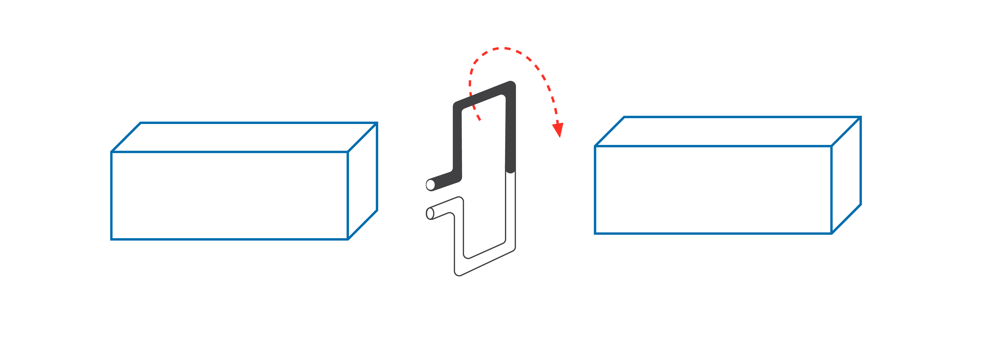
Consider a square loop moving at constant speed into a uniform magnetic field, as shown below. Recall that in diagrams, magnetic field lines are typically represented with crosses (×) for fields directed into the page, and with arrows pointing from the north to the south pole of a magnet.
Interact with the diagram for explanations of how the loop moving into the magnetic field affects the magnetic flux.
Loop rotating in a magnetic field
A loop rotating within a magnetic field experiences a continuously changing magnetic flux. In this setup, the loop is stationary in space but spins about an axis, typically perpendicular to a uniform magnetic field.
As the loop rotates, the angle between the magnetic field and the loop's surface area changes over time. This causes the perpendicular component of the magnetic field—and therefore the magnetic flux through the loop—to vary along a sine wave. Click on the diagram below to for explanations of how the loop rotating in a magnetic field affects the magnetic flux.
Faraday’s law
Electromotive force, or emf, is the voltage generated in a circuit due to a changing magnetic environment. When the magnetic flux through a wire loop changes, an emf is induced. If the circuit is complete, this emf drives a current through the loop.
In practice, emf is often generated by rotating a loop within a magnetic field, as in electrical generators. However, any change in magnetic flux can induce an emf.
Consider a stationary magnet is next to a wire loop, as shown below
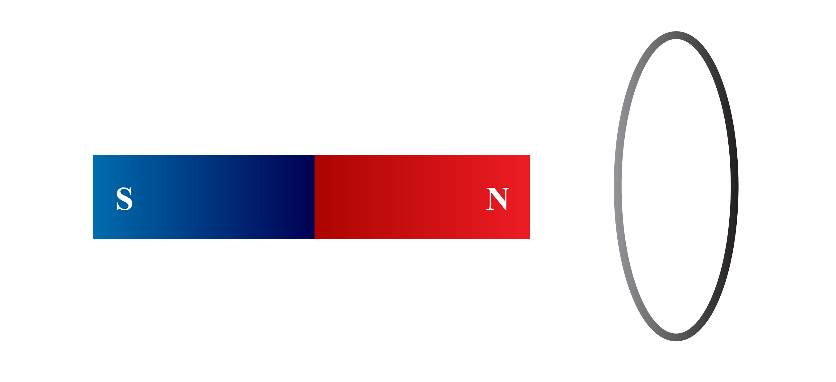
In this setup, the magnet creates a magnetic field that passes through the wire loop, resulting in a constant magnetic flux. However, since neither the magnet nor the loop is moving, there is no change in flux. Thus, no emf is induced and no current flows in the loop.
Now, consider the magnet is moving towards the wire loop as shown.
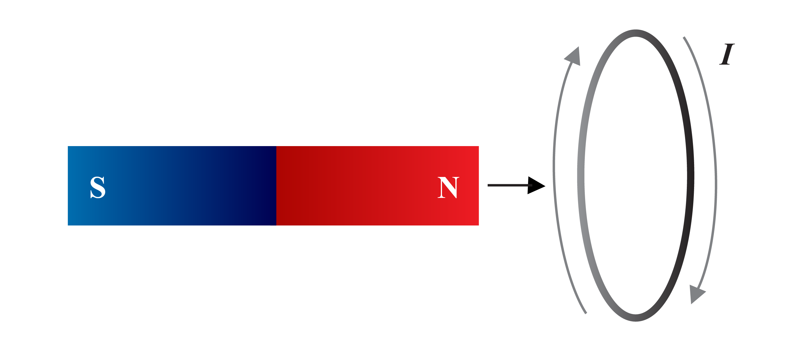
The magnet produces a magnetic field that passes through the loop – there is magnetic flux.
As the magnet approaches the loop, the strength of the flux increases – there is a change in flux. Hence an electric current is induced in the loop.
The size of the emf induced in the loop is quantified by Faraday’s law.
\[ \varepsilon = -N \frac{\Delta \Phi}{\Delta t} \]
Where:
- \(\varepsilon\) is the induced emf (\(\text{V}\))
- \(N\) is the number of turns or coils in the loop
- \(\Delta \Phi\) is the change in magnetic flux (\(\text{Wb}\))
- \(\Delta t\) is the change in time
NoteThe negative sign in Faraday’s law is a reminder of the direction of the induced emf. This is further unpacked in the next section on Lenz’s law. When calculating the induced emf, this negative sign can be ignored. |
Worked Example
Determine the size of the induced emf in a single circular loop of radius \(5\text{ cm}\) as it moves from a region with a magnetic field of \(0 \text{ T}\) to a region with magnetic field strength of \(2.0 \times 10^{-4} \text{ T}\) in a time of \(0.25\) seconds.
Determine the area of the circular loop.
\[ A = \pi r^2 = \pi \times (0.05)^2 = 7.85 \times 10^{-3} \ \text{m}^2 \]
Calculate the change in magnetic flux.
Initial flux \(\Phi_B = BA = 0 \times 7.85 \times 10^{-3} = 0\ \text{Wb}\)
Final flux \(\Phi_B = BA = 2.0 \times 10^{-4} \times 7.85 \times 10^{-3} = 1.57 \times 10^{-6} \ \text{Wb}\)
\[\begin{align*} \Delta \Phi_B &= 1.57 \times 10^{-6} - 0 \\ &= 1.57 \times 10^{-6} \ \text{Wb} \end{align*}\]
Use Faraday’s law, disregarding the negative sign.
\[ \begin{align*} \varepsilon &= N \frac{\Delta \Phi}{\Delta t} \\ &= 1 \times \frac{1.57 \times 10^{-6}}{0.25} \\ &= 6.28 \times 10^{-6} \ \text{V} \ \text{ or } 6.28 \mu \text{ V} \end{align*} \]
Check your understanding
View
Graphing induced emf
As the induced electromotive force (emf) is directly related to the rate of change of magnetic flux, as described by Faraday’s law, then:
- Mathematically, emf is the negative rate of change of flux over time.
- Graphically, emf is the negative of the gradient(slope) of the \(\Phi -t\) graph.
Consider again, the instance when a square loop passes into a magnetic field:

The graph of the flux was given by:
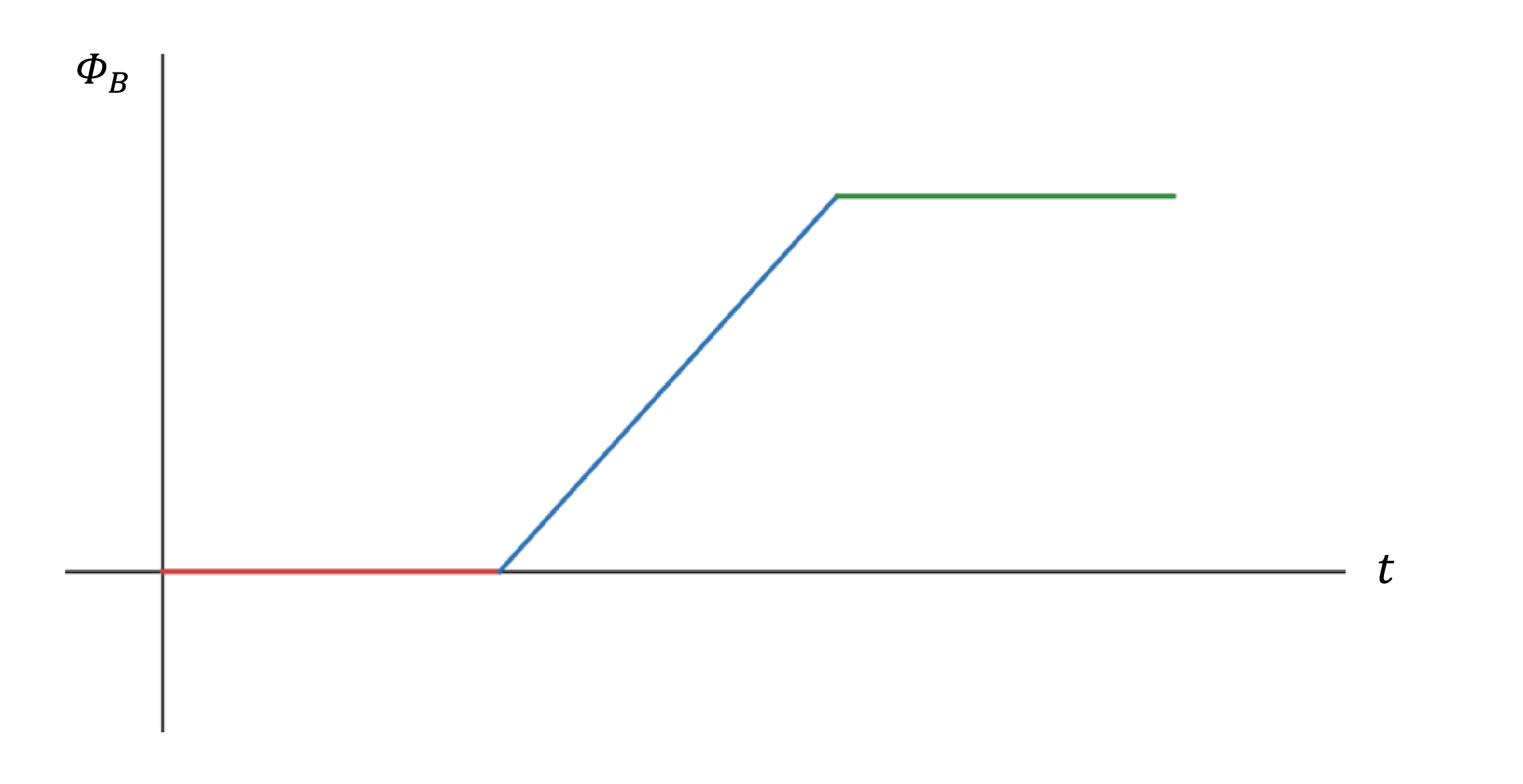
To determine the graph of the induced emf, take the negative of the gradient of the \(\Phi -t\) graph, as plotted below.
Now consider again the case where a loop is rotating in a magnetic field.
The graph of the flux was given by:

To determine the graph of the induced emf, again we take the negative of the gradient of the \(\Phi -t\) graph, as plotted below.
This relationship between magnetic flux and induced emf can be understood mathematically using calculus.
If the \(\Phi -t\) graph is one period of a cosine graph, and emf is the negative rate of change of magnetic flux, then:
\[
\varepsilon = -\frac{d}{dt} (\cos t) = -(-\sin t) = \sin t
\]
Thus, if the \(\Phi-t\) graph follows a cosine shape, then the corresponding \(\varepsilon-t\) graph will follow a sine curve. This phase difference between emf and flux is a key feature of alternating current (AC) generation.
Worked Example
A single circular loop of area \(2\text{ cm}^{2}\) is immersed in a uniform magnetic field of strength \(5.0\text{ mT}\). If the loop is rotated at a rate of one rotation per second, determine the magnitude of the average emf produced in a quarter rotation.
Solution
- Determine the change in flux \(\Delta \Phi\)
A quarter rotation will take the loop from being perpendicular to the field to parallel to it, or vice versa. Thus, the flux will go from a maximum to zero, or from zero to a maximum. Therefore, assuming either parallel or perpendicular to be the starting point will yield the same magnitude of average emf.
Assume starting parallel.
Initial \(\Phi = B \times A = 0 \times 0.02 = 0 \ \text{Wb}\)
Final \(\Phi = B \times A = 0.005 \times 0.02 = 1 \times 10^{-4} \ \text{Wb}\) - Determine the time \(\Delta t\).
A full rotation is 1 second, hence a quarter rotation is \(\Delta t = 0.25 \text{ s}\) - Use Faraday’s law.
\[ \varepsilon = N \frac{\Delta \Phi}{\Delta t} = 1 \times \frac{10^{-4} - 0}{0.25} = 4 \times 10^{-4} \ \text{V} \quad \text{or} \quad 400\,\mu\text{V} \]