Area estimation techniques
Estimating the area under a curve is a practical method to approximate an area when an exact answer is not required. This process often involves using simple shapes, like rectangles or trapeziums, to approximate the area between the curve and the \(x\)-axis. However, these shapes can either overestimate or underestimate the true area, leading to some error. Increasing the number of shapes and reducing their width improves the accuracy of the estimate.
Use this page to revise the three commonly used techniques for estimating the area under the curve:
Left endpoint method
In the left endpoint method, the area under a curve is approximated by by the calculating the total area of a series of rectangles. Each rectangle is of equal width, and the height of each rectangle is determined by the value of the function at its left endpoint.
The general formula for the left endpoint method is:
\[A_{L} = \frac{b-a}{n}[f\left(x_{0}\right) + f\left(x_{1}\right) + \cdots + f\left(x_{n - 1}\right)]\]
Where \(n\) is the number of rectangles used to approximate the area under the curve between \(x=a\) and \(x=b\).
That is, the rectangle of each subinterval \(\left[x_{i-1}, x_i\right]\), for \(i=1,2, \ldots, n\), has a width of \(\Delta x=\frac{b-a}{n}\). The height of each rectangle is given by \(f\left(x_{i-1}\right)\). Thus, the area of each rectangle is \(f\left(x_{i-1}\right) \Delta x\), and summing these gives the total approximate area.
![Graph of f(x) from x=a to x=b, detailing the left endpoint method for approximating the area under a curve. A series of n rectangles are drawn below a curve, f(x). Each rectangle is drawn from interval [x_{n-1}, x_n], and so has a width of (a-b)/n. Each rectangle has a height determined by the value of the function at its left endpoint, that is, f(x_{n-1}.](https://www.monash.edu/__data/assets/image/0006/4146522/D11_Area-Estimation-Techniques_Extra.png)
The left endpoint method provides an overestimate if the function is strictly decreasing.
The left endpoint method will produce an underestimate for an increasing function.
Worked Example
Approximate the area under the curve \(f(x)=1-\dfrac{1}{4} x^2\) between \(x=0\) and \(x=2\) using left endpoint method:
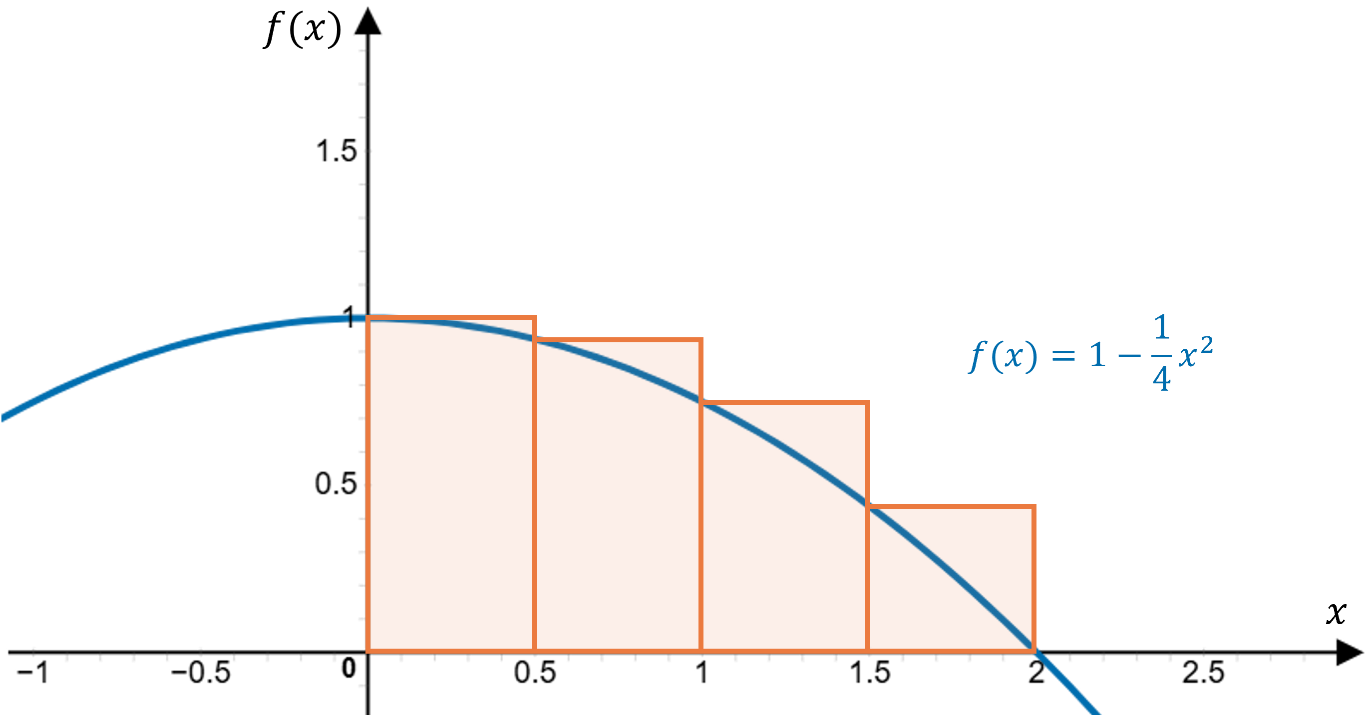
Estimate the area under the curve by finding the area \(\text{base} \times \text{height}\) of each rectangle:
\[\begin{aligned}A_L & = \frac{b-a}{n}\left[f\left(x_0\right)+f\left(x_1\right) + f\left(x_2\right)+ f\left(x_3\right) \right] \\& = \frac{2-0}{4} \left[f(0)+f(0.5)+f(1)+f(1.5) \right] \\& =0.5 \times f(0)+0.5 \times f(0.5)+0.5 \times f(1)+0.5 \times f(1.5) \\& =0.5 \times \left(f(0)+f(0.5)+f(1)+f(1.5)\right) \\& =0.5 \times\left(1+\frac{15}{16}+\frac{3}{4}+\frac{7}{16}\right) \\& =\frac{25}{16}=1.5625 \text { square units }\end{aligned}\]
Note the actual area is \(\frac{5}{3}\approx 1.33\) square units. In this case, the left endpoint method gives an overestimate as the top edge of each rectangle crosses the actual curve, covering more area than the curve itself.
Right endpoint method
In the right endpoint method, the area under a curve is also approximated by calculating the total area of a series of rectangles. Again each rectangle is of equal width, but the height of each rectangle is determined by the value of the function at its right endpoint.
The general formula for the right endpoint method is:
\[A_{R} = \frac{b - a}{n}[f\left(x_{1}\right) + f\left(x_{2}\right) + \cdots + f\left(x_{n}\right)]\]
Where \(n\) is the number of rectangles used to approximate the area under the curve between \(x=a\) and \(x=b\).
That is, the rectangle of each subinterval \(\left[x_{i-1}, x_i\right]\), for \(i=1,2, \ldots, n\), has a width of \(\Delta x=\frac{b-a}{n}\). The height of each rectangle is given by \(f\left(x_{i}\right)\). Thus, the area of each rectangle is \(f\left(x_{i}\right) \Delta x\), and summing these gives the total approximate area.
The right endpoint method provides an underestimate if the function is strictly decreasing.
The right endpoint method will produce an overestimate for an increasing function.
Worked Example
Approximate the area under the curve \(f(x)=1-\frac{1}{4} x^2\) between \(x=0\) and \(x=2\) using right endpoint method:
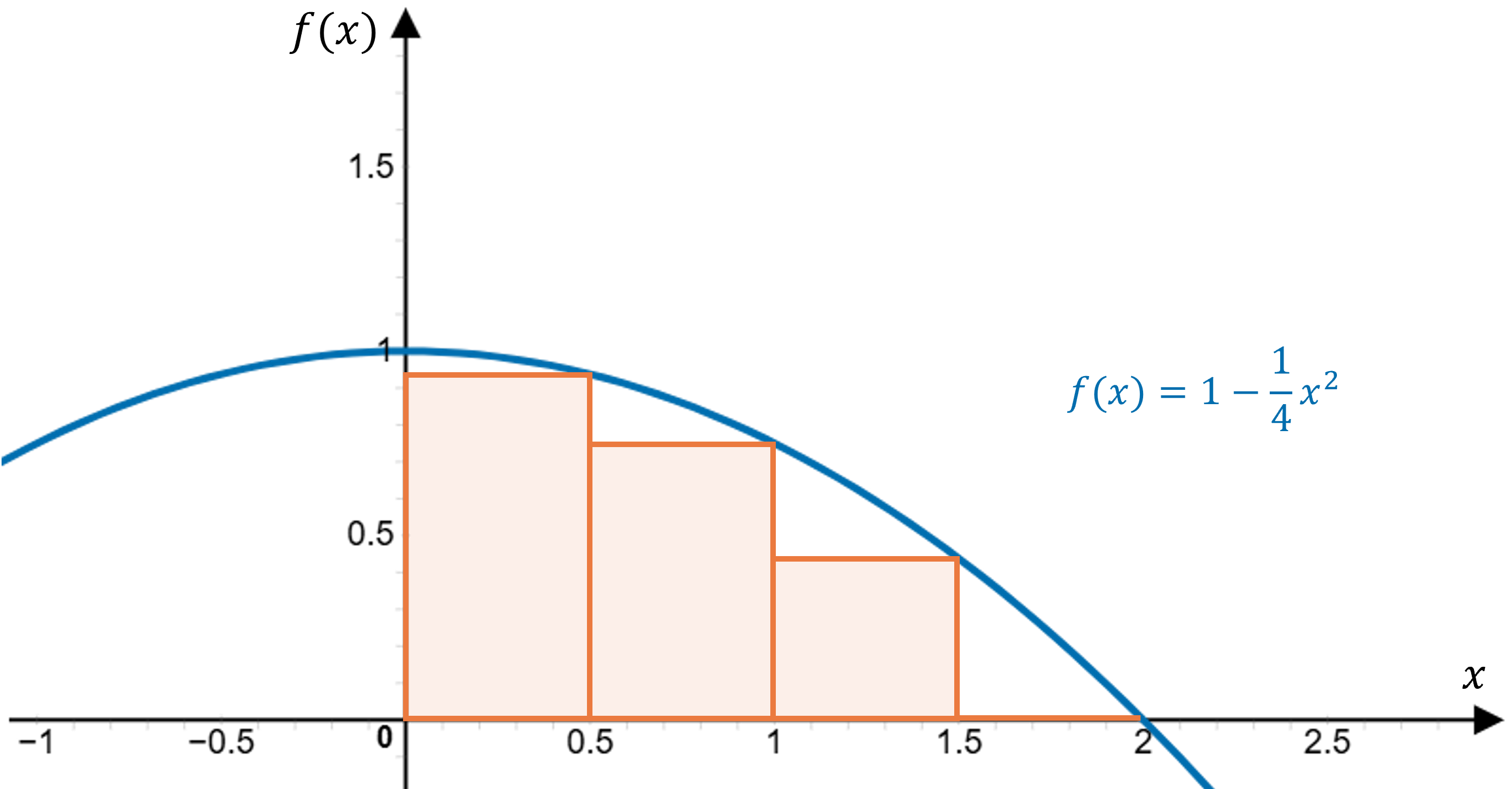
Estimate the area under the curve by finding the area \(\text{base} \times \text{height}\) of each rectangle:
\[\begin{aligned}A_R & = \frac{b-a}{n}\left[f\left(x_1\right)+f\left(x_2\right) + f\left(x_3\right)+ f\left(x_4\right) \right] \\& = \frac{2-0}{4} \left[f(0.5)+f(1)+f(1.5)+f(2)\right] \\& =0.5 \times f(0.5)+0.5 \times f(1)+0.5 \times f(1.5)+ 0.5 \times f(2)\\& =0.5 \times\left(f(0.5)+f(1)+f(1.5)+f(2)\right) \\& =0.5 \times\left(\frac{15}{16}+\frac{3}{4}+\frac{7}{16}+0\right) \\& =\frac{17}{16}=1.0625 \text { square units }\end{aligned}\]
Note the actual area is \(\frac{5}{3} \approx 1.33\) square units. In this case, the right endpoint method gives an underestimate as the top edge of each rectangle does not cross the actual curve, covering less area than the curve itself.
Trapezium method
In the trapezium method, the area under a curve is closely approximated by calculating the total area of a series of trapeziums. Each trapezium is of equal height, and the lengths of the two parallel sides of the trapezium are determined by the value of the function.
The general formula for the trapezium method is:
\[A_T=\frac{b-a}{2 n}\left[f\left(x_0\right)+2 f\left(x_1\right)+2 f\left(x_2\right)+\cdots+2 f\left(x_{n-1}\right)+f\left(x_n\right)\right]\]
Where \(n\) is the number of trapeziums used to approximate the area between \(x=a\) and \(x=b\).
That is, the trapezium of each subinterval \(\left[x_{i-1}, x_i\right]\) (for \(i=1,2, \ldots, n\) ) has a height of \(\Delta x=\frac{b-a}{n}\). \(a\) and \(b\) represent the lengths of the parallel sides and correspond to the function values \(f\left(x_{i-1}\right)\) and \(f\left(x_i\right)\) respectively, while \(h\) represents the height, which in this context is the width of the subinterval \(\Delta x\).
The trapezium method finds an area closer to the true area under the curve, when compared to the left and right endpoint methods.
Worked Example
Approximate the area under the curve \(f(x)=1-\frac{1}{4} x^2\) between \(x=0\) and \(x=2\) using the trapezium method:
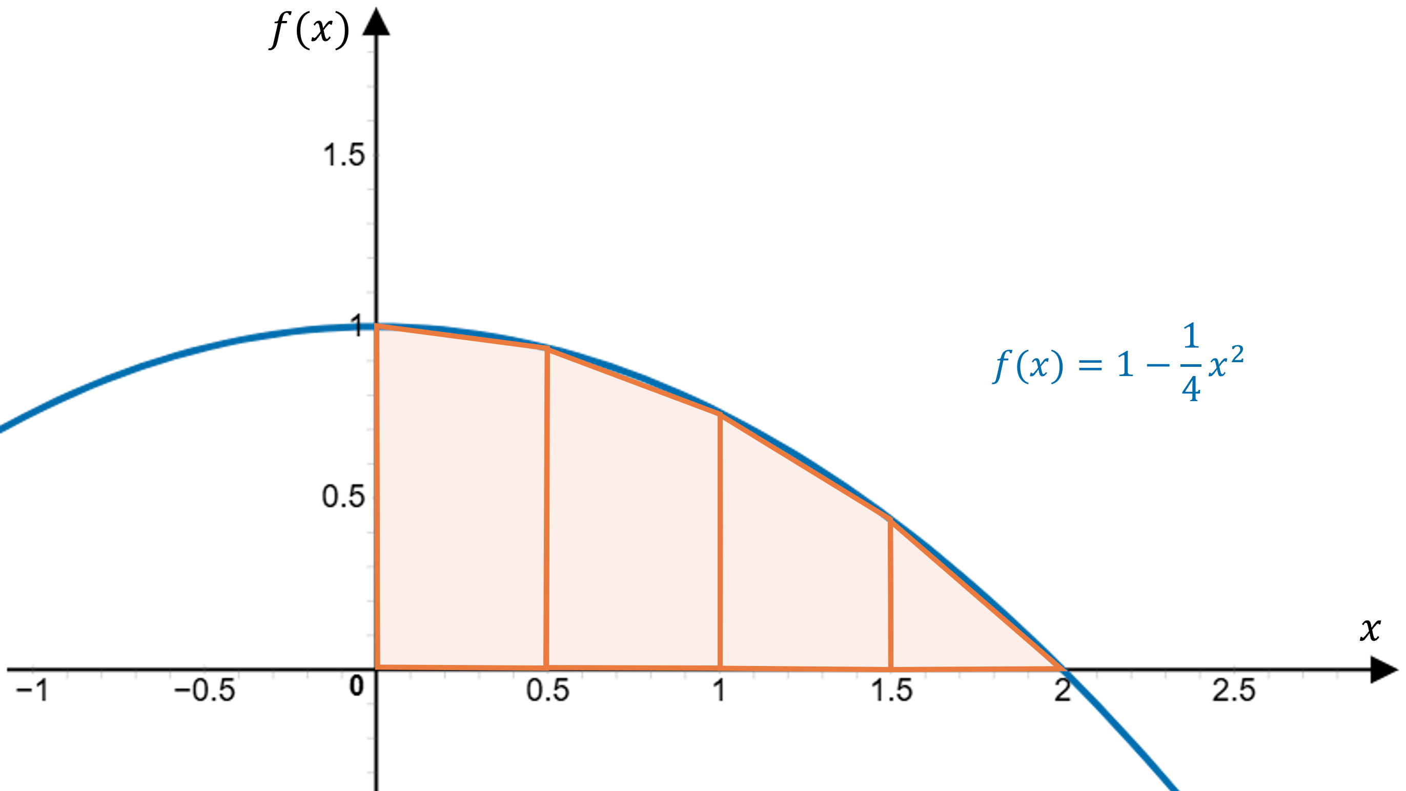
By finding the area \(\frac{1}{2}\times {sum of two parallel side lengths} \times h\) of each trapezium:
\[\begin{aligned}A_t =& \frac{b-a}{2 n}\left[f\left(x_0\right)+2 f\left(x_1\right)+2 f\left(x_2\right)+2 f\left(x_{3}\right)+f\left(x_4\right)\right]\\= & \frac{2-0}{2\times 4} \left[f(0)+2f(0.5)+2f(1)+2f(1.5) +f(2) \right] \\= & \frac{1}{2} \times 0.5 \times(f(0)+f(0.5))+\frac{1}{2} \times 0.5 \times(f(0.5)+f(1)) \\& +\frac{1}{2} \times 0.5 \times(f(1)+f(1.5))+\frac{1}{2} \times 0.5 \times(f(1.5)+f(2)) \\= & \frac{1}{2} \times 0.5 \times(f(0)+2 f(0.5)+2 f(1)+2 f(1.5)+f(2)) \\= & \frac{1}{2} \times 0.5 \times\left(1+\frac{15}{8}+\frac{3}{2}+\frac{7}{8}+0\right) \\= & \frac{21}{16}=1.3125 \text { square units }\end{aligned}\]
Note the actual area is \(\frac{5}{3} \approx 1.33\) square units. The trapezium method is a slight underestimate in this case, but more accurate than either the left or right endpoint methods.
