Solving linear equations and inequalities
Linear functions are used to model a broad range of real-world problems. The ability to solve linear equations and inequalities is an essential skill for analysing these models. This section covers methods to solve linear equations and inequalities both algebraically and graphically, as well as translating worded problems into linear equations, providing the necessary tools to address various mathematical and practical challenges.
Use this page to revise the following concepts of linear equations and inequalities:
- Solving linear equations
- Solving linear inequalities
- Translating worded problems into linear equations
Solving linear equations
Linear equations
A linear equation is an equation that, when graphed, forms a straight line. The general form for a linear equation is \(y = a + bx\) where \(a\) is the \(y\)-intercept and \(b\) is the gradient or slope.
Key features of a linear equations are:
- It has one or more variables
- all variables are raised to the power of \(1\)
- no variables are multiplied with one another
- variables are not arguments of more complex functions, such as \(\sin{(x)}\) or \(\log{(x)}\).
A linear equation can have more than one variable, such as \(y = a + bx +cz\); however, this resource focuses on equations involving one or two variables.
Linear equations can be represented in different forms, for example:
- \(y = 4x + 9\)
- \(3x - 2.8y = 54\)
- \(2(x - 5) = 6y\)
- \(\frac{y}{3} = \frac{4}{7}x +1\)
- \(x = -5\)
- \(y = 0.1\)
- \(y = \sin(4)x\)
Examples of equations that are not linear:
- \(xy = 64\)
- \(y = 14 - x^2\)
- \(y = \sqrt{x}\)
- \(x^2 = y^2 = 25\)
- \(y = \sin(4x)\)
Solving a linear equation means finding the value of an unknown variable that satisfies the equation. Often, this involves using the value of a known variable to determine the value of an unknown variable.
- Given \(x\), solve for \(y\): Substitute the value of \(x\) into the equation to find \(y\).
- Given \(y\), solve for \(x\): Rearrange the equation to isolate \(x\).

Linear equations can be solved algebraically and graphically.
Worked Example
Solve for \(x\) in the equation \(y =\frac{5}{2}x - 20\) when \(y = 10\).
| Solving for \(x\) algebraically | Solving for \(x\) graphically |
|---|---|
Substitute \(y = 10\) into the equation: \[10 = \frac{5}{2}x - 20\] Add 20 to both sides to isolate the term with \(x\): \[30 = \frac{5}{2}x\] Multiply both sides by 2 to eliminate the fraction: Divide both sides by 5 to solve for \(x\): Note the last two steps can be combined into a single step by multiplying both sides of the equation by \(\frac{2}{5}\). |  |
 Check your understanding
View
Check your understanding
View

Solving linear inequalities
A linear inequality is similar in form to a linear equation, but the equal sign is replaced by an inequality symbol (\(>\), \(<\), \(\ge\), or \(\le\)).
Unlike typical linear equations, which usually have a single solution, the solution to a linear inequality typically consists of a range of values. Solving an inequality means finding all possible values of the variables that make the inequality true. This typically involves rearranging the inequality—much like solving an equation—to isolate the variable. However, unlike an equation that may have a single solution or a finite set of solutions, the result here is a continuous set or range of values. These inequalities commonly emerge in contexts that use terms like "at least" or "at most."
Representing linear inequalities on a number line
| Linear inequality | Corresponding representation on a number line |
|---|---|
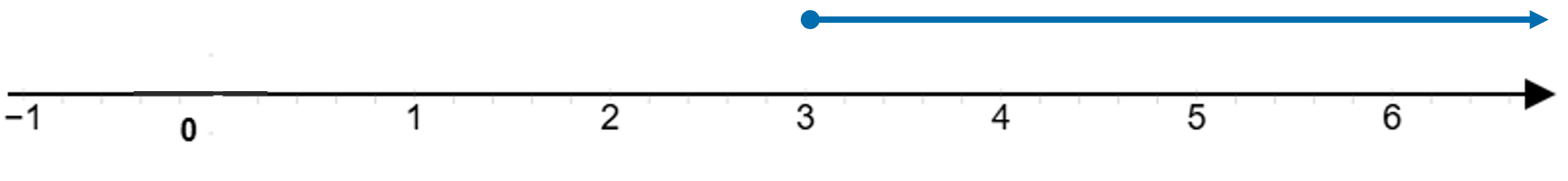
\[x > 3\] The circles is open as \(x \neq 3\). |
|
\[x \geq 3\] The circle is closed as \(x\) is greater than and equal to \(3\). |
|
\[x \leq -3\] The circle is closed as \(x\) is less than and equal to \(3\). | 
|
|
\[-3 < x \leq 3\] The left circle is open, as \(x \neq -3\), the right circle is closed as \(x\) includes \(3\). | 
|

Solving linear inequalities
Inequalities are generally solved using the same steps as for equations, except when multiplying or dividing both sides of an inequality by a negative number, in which case you must reverse the direction of the inequality sign.
This is because when you multiply or divide both sides by a negative number, all positive values become negative, and all negative values become positive, reversing their positions on a number line.
Consider the case where \(x =2\) and \(y = 3\). In this case, \(y\) is larger than \(x\), so we write this as \(x < y\). However, if we multiply \(x\) and \(y\) by \(-\)1, we get\(-x = -2\) and \(-y=-3\). In this case, \(-x\) is larger than \(-y\), so we flip the direction of the inequality sign: \(-x > -y\).
Worked Example
Solve for \(x\) in the inequality \(-3x + 5 \geq 11\).
Solution
Subtract 5 from both sides:
\(-3x \geq 6\) inequality sign does not change direction when adding or subtracting a number
Divide both sides by −3:
\( x \leq -2\) inequality sign reverses direction when multiplying or dividing by a negative number
Representing linear inequalities on a plane
When graphing a linear inequality on a coordinate plane, we:
- shade the region containing all points that make the inequality true
- use a solid boundary line if the edge points are included (inequalities with \(\le\) or \(\ge\))
- use a dashed boundary line if the edge points are excluded (inequalities with \(<\) or \(>\)).
Steps for graphing a linear inequality on the coordinate plane:
- Graph the boundary line of the inequality
- Determine if the boundary line is included (use a solid line) or excluded (use a dashed line)
- Select a point not on the boundary line to determine which side of the line to shade.
Worked Examples
Example 1
Sketch the graph of the inequality \(y > 2\).
| Working steps | Graph |
|---|---|
1. Graph the boundary line \(y=2\) 2. Since the inequality is \(>\) a dashed line is used, as the points on the line are not included in the solution set. 3. Select a point not on the boundary line: \((1,1)\) Substitute \(y=1\) into the inequality \(1 \neq 2\) The inequality is false, therefore the required region is the opposite side. |
|

Example 2
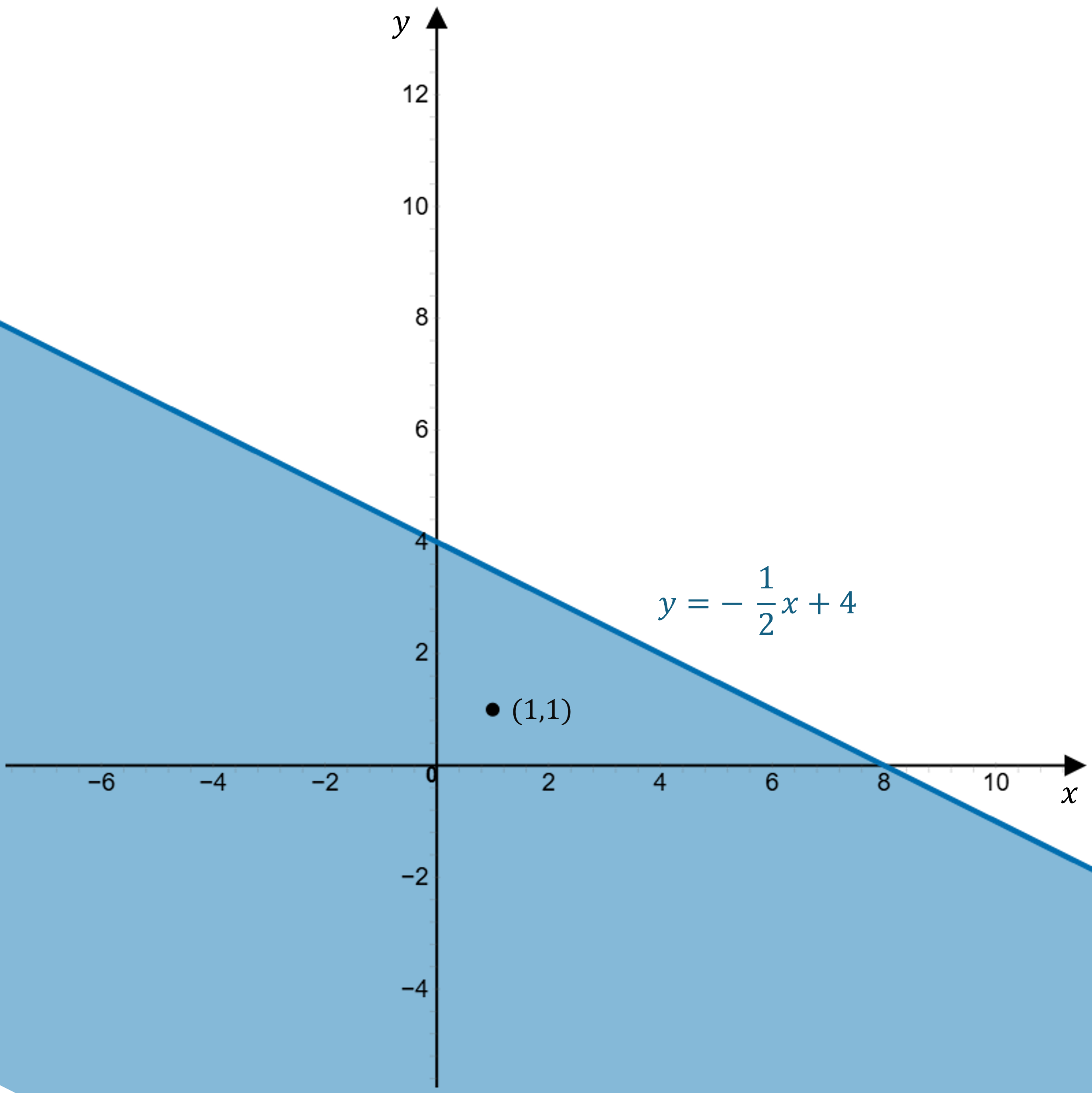
Sketch the graph of the inequality \(y \leq -\frac{1}{2}x + 4\).
| Working Steps | Graph |
|---|---|
1. Graph the boundary line \(y = -\frac{1}{2}x + 4\). 2. Since the inequality is \(\leq\) a solid line is used, as the points on the line are included in the solution set. 3. Select a point not on the boundary line:\[(1,1)\] Substitute \(x = 1\) and \(y = 1\) into the inequality \[\begin{align}1 &\leq -\frac{1}{2}(1) + 4 \\ 1 &\leq 3\frac{1}{2} \end{align}\] The inequality is true, therefore the required region is on the side containing the test point. |
|
Check your understanding
View
Translating worded problems into linear equations
Linear equations are used to model relationships in real-world scenarios where two variables change at a constant rate. Common examples include calculating wages based on an hourly rate, determining total costs with fixed and variable components, or computing simple interest on savings over time.
Translating worded problems into linear equations requires interpreting the problem, identifying key elements, and expressing the relationships mathematically.
Steps for formulating linear equations
- Read the problem: Carefully interpret the problem to understand the situation and what is being asked.
- Highlight key information: Identify constants, rates, quantities, and any relationships explicitly stated or implied.
- Define variables: Assign symbols (e.g. \(x\), \(y\)) to unknowns, clearly stating what each represents.
- Identify relationships: Determine how the variables are connected, noting proportionality, fixed amounts, or other dependencies.
- Formulate the linear equation: Translate the identified relationships into a mathematical equation.
- Check your linear equation: Substitute a pair of values into the linear equation to check for accuracy.
Worked Example
A plumber charges a call-out fee of \(\$70\) and \(\$85\) per hour of work.
- a) Write a linear equation to represent the total cost \((C)\) in terms of the hours worked \((h)\).
b) Determine the total cost if the plumber works for \(3.5\) hours.
Example solution
Read the Problem:
The plumber's charges include a fixed call-out fee and an hourly rate.
Highlight key information:
Call-out fee: \(\$70\) (fixed cost)
Hourly rate: \(\$85/\text{hour}\)
Define variables:
C represents the total cost
h represents the number of hours worked
Identify relationships
The total cost \(C\) is the sum of the fixed call-out fee, \(\$70\), and the cost of the hours worked.
Formulate the linear equation:
\(\$85\) per hour translates to \(85\times h\)
\(C = 85h + 70\)
Check your linear equation:
The cost of \(1\) hour’s work is \($70 + $85 = $155\)
Check the formula by substituting in \(h = 1\)
\[\begin{align}C &= 85(1) + 70 \\ C &= 155\end{align}\]
Solution for b):
Substitute \(h = 3.5\) into the equation to determine the total cost for \(3.5\) hours of work.
\[\begin{align}C &= 85(3.5) + 70 \\ C &= \$367.50\end{align}\]