Continuous random variables
A continuous random variable is a type of variable that can take on any value within a given range. Unlike discrete random variables, which have a countable number of outcomes, continuous random variables can assume infinitely many values, usually within an interval on the real number line. These variables are especially useful in situations where measurements are involved—such as time, length, or temperature—because the possible values are not limited to specific points. For example, height could be to the nearest centimetre (163 cm), to a tenth of a centimetre (163.6 cm) or hundredth of a centimetre (163.68 cm). Understanding continuous random variables is essential in statistics, as they form the foundation for modelling and analysing real-world data that varies smoothly rather than in steps.
Use this page to revise the following concepts regarding continuous random variables:
Probability Density Function
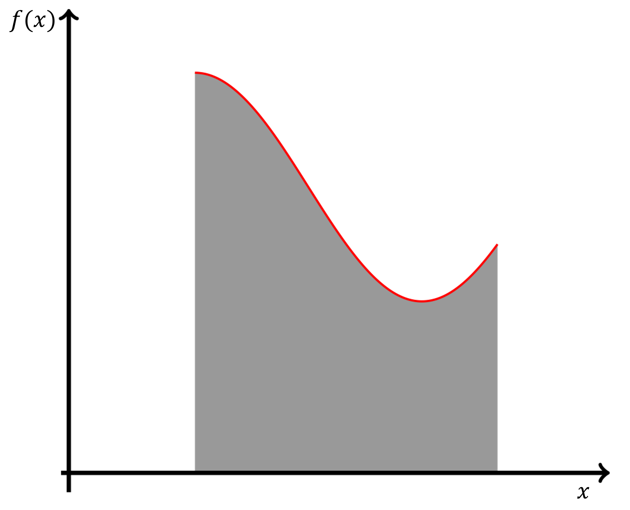
Calculating probabilities for continuous random variables requires a different approach from the methods used with discrete variables. If all the outcomes of a continuous random variable are displayed in a histogram, the interval widths become infinitely small. Thus, instead of counting outcomes as we might with discrete random variables, we use area under the curve to represent probability. The area under a smooth curve gives the probability of values falling within a certain range and is found by taking the definite integral of a probability density function. This curve is called the probability density function (PDF), and it describes the probability distribution of a continuous random variable, often denoted as \(X\). The variable \(x\) represents a specific value that \(X\) might take, and \(f(x)\) gives the value of the PDF at that point.
There are two key conditions that any probability density function (PDF) must satisfy:
- The function must always be non-negative, since probabilities cannot be less than zero
- The total area under the curve must equal 1, representing the fact that the probability of some outcome occurring within the entire range is certain.
These conditions ensure the PDF correctly models a valid probability distribution for a continuous random variable.
To find the probability of a particular interval, the area under the curve between the interval must be found.
\[\Pr\left(a< X< b\right)=\int_{b}^{a}f\left(x\right)dx \]

Importantly, many probability density functions may be represented by piecewise functions, where different rules apply to different intervals of \(x\). For example,
\[f\left(x\right)=\begin{cases} &\frac{\pi}{20}\sin\left(\frac{\pi(x-7)}{10}\right), &7 \leq x\leq 17 \\ &0, &\text{otherwise} \end{cases} \]
Check your understanding
View

The Mean
Just like with discrete random variables, we can calculate the expected value (or mean) of a continuous random variable to find its long-run average value over many trials. In the continuous case, this is done using an integral rather than a summation. The formula is
\[E\left(X\right)=\int_{-\infty}^{\infty}xf\left(x\right)dx\]
However, in most practical cases, the PDF is only nonzero over a finite interval. The limits of integration are then adjusted to reflect the domain where \(f(x)>0\). For example, if your PDF is only defined between \(a\) and \(b\), the mean is:
\[E\left(X\right)=\int_{a}^{b}xf\left(x\right)dx\]
Check your understanding
View
Percentiles and the Median
Percentiles are values of the random variable \(X\) that divide the area under the probability density function into specified proportions. In other words, the \(p-th\) percentile is the value \(q\) such that the probability that \(X\) is less than or equal to \(q\) is \(p\). To find any percentile, we solve the equation:
\[\int_{-\infty}^{q}f\left(x\right)dx=p\]
Where:
- \(p\) is the desired percentile expressed as a decimal,
- \(q\) the value of \(X\) that marks the boundary for that cumulative area.
For example, the value of \(q\) such that 25% of the outcomes lie below it is called the 25th percentile. It satisfies:
\[\int_{-\infty}^{q}f\left(x\right)dx=0.25\]
Percentiles are useful for interpreting the distribution of values, especially when identifying cut-offs for central ranges or extremes.
The median is one such useful percentile. The median is another important measure of central tendency. It represents the value that divides the probability distribution into two equal halves. In other words, 50% of the probability lies below the median, and 50% lies above.
Since the median is the 50th percentile, we can find it by solving:
\[\int_{-\infty}^{m}f\left(x\right)dx=0.5\]
Where \(m\) is the value of \(X\) such that the area under the probability density function up to m is \(0.5\).
The median is especially useful when the distribution is skewed, as it is not affected by extreme values in the same way the mean is.
Check your understanding
View
Variance and Standard Deviation
Variance and standard deviation are measures of how spread out the values of a continuous random variable are around the mean.
The variance of a continuous random variable \(X\) is defined as the expected value of the squared difference from the mean:
\[VAR\left(X\right)=E\left(\left(X-\mu\right)^2\right)\]
This can also be calculated more easily using the shortcut formula:
\[VAR\left(X\right)=E\left(X^2\right)-\left(E\left(X\right)\right)^2\]
The standard deviation is the square root of the variance:
\[SD\left(X\right)=\sqrt{VAR\left(X\right)}\]