Basic probability
Probability is a fundamental concept in mathematics and statistics that deals with the likelihood of events occurring. It provides a framework for quantifying uncertainty and making predictions based on known information. This section explores the foundational ideas of probability, starting with elementary events and their basic properties.
Use this page to revise the following concepts within basic probability:
- Sample space and the probability of events
- Elementary Events
- Compound Events
- Venn diagrams
- Mutually Exclusive
- Addition Rule
- Conditional Probability
- Independence
- Tree Diagrams
- Law of Total Probability
- Probability Tables
Sample space and the probability of events
We call the collection of all possible outcomes for an experiment or trial the sample space, often written as \(\varepsilon\) (and sometimes as \(S\)).
In probability, an event is a collection of one or more possible outcomes of an experiment or trial that represents a specific result, such as rolling a 3 on a six-sided die, or meets a particular condition, such as rolling an even number.
The measure of likelihood of the event occurring is the probability of the event. It is calculated as a number between 0 and 1, where 0 means the event is impossible and 1 means the event is certain.
If the outcomes are presumed to be equally likely, the probability of event \(A\), is found by:
\[\Pr(A) = \frac{n(A)}{n(\varepsilon)} \]
Where:- \(\Pr(A)\) is the probability of event \(A\) occurring.
- \(n(A)\) is the number of possible outcomes matching event \(A\).
- \(n(\varepsilon)\) is the total number of possible outcomes.
There are two central rules of probability. The first is that probability is always positive.
\[0\le \Pr{\left(A\right)}\le1\]
Secondly, the sum of the probabilities of all possible outcomes is \(1\). This is represented by:
\[\sum \Pr\left(x\right)=1\]
Worked Example
A 10-sided die numbered 1 to 10 is rolled once. What is the probability that the upper most number is less than 6?
For a 10-sided die, there are 5 out of the possible 10 outcomes that would be successful. That is, that would have an upper most number of less that 6. Therefore:
\[\begin{align} &n(A)=5 \\ &n(\varepsilon)=10 \end{align}\]
The probability of this outcome can then be calculated as:
\[\Pr(A) = \frac{\text{The number of }A}{\text{The total number}}=\frac{n(A)}{n(\varepsilon)} =\frac{5}{10}=\frac{1}{2}\]
The probability of a number less than 6 being rolled on 10-sided die is \(\frac{1}{2}\). Or, half of the rolls of a 10-sided die would roll a number less than 6.
 Check your understanding
View
Check your understanding
View

Elementary Events
An elementary event is a single, specific outcome of an experiment. It may also be called a simple event. For a simple experiment like rolling one fair die, each outcome (e.g. rolling a 4) is an elementary event.
If event \(B\) is an elementary event, then the number of outcomes of event \(B\) , or \(n(B)\) must be equal to \(1\). In a finite sample space with equally likely outcomes, the probability of an elementary event is therefore:
\[\Pr(B) = \frac{1}{n(\varepsilon)} \]
Compound Events
Compound events involve two or more simple events within the same sample space. Instead of focusing on a single outcome, a compound event considers multiple outcomes happening together or separately. These events could be more than one property of an outcome of a simple experiment (e.g., the probability of drawing a card from a deck that is both red and lower than a 5), or combining outcomes of more than one trial (e.g., several flips of a coin or rolls of a die). There are several key terms that are used to describe the potential relationships between compound events.
Intersection
The event that both \(A\) and \(B\) occur, when \(A\) and \(B\) are two events in the sample space \(\varepsilon\). This intersection between the events is represented by:
We read this as "\( A \text{ intersection }B\)".
If the events are independent, that is, one event does not affect the outcome of the other event, then we can calculate this as
\[\Pr(A\cap B)=\Pr(A)\times \Pr(B)\]
This formula may differ for conditional probability, and when one event is a subset of the other (if \(B\subset A \)).
If \(B\subset A\), then
\[\Pr(A\cap B) = \Pr(A)\]
For example, if \(A\) the probability of drawing 4 aces from a deck of card and \(B\) is the probability of drawing at least 2 aces from a deck of cards, then then if \(A\) happens, \(B\) must also happen.
Union
The event that \(A\) or \(B\) or both occur, when \(A\) and \(B\) are two events in the sample space \(\varepsilon\). This union between the events is represented by:
We read this as "\(A\text{ union }B\)".
We can calculate the probability of a union of events as
\[\Pr(A\cup B)=\Pr(A)+\Pr(B)-\Pr(A\cap B)\]
Complementary
Two events are complementary if exactly one of the events must occur. For event \(B\), the complementary event is \(B^\prime\) (read as "\(\text{not }B\)"). As either the event, or its complement, must occur, then:
Venn diagrams
A Venn diagram visualises the sample space and illustrates how all the elements are distributed among the events. In a Venn Diagram, the sample space is represented by a rectangle, and events are represented by, usually overlapping, circles within that rectangle. A Venn diagram helps you to easily depict relationships including union, intersection and complement.
For example, say you have a sample space of 20 students who may study mathematics (event \(M\)) or physics (event \(P\)). 15 student study maths, 9 study physics, 5 students study both maths and physics \((A\cap B)\) and 1 does not study either mathematics or physics. This information would be displayed in a Venn diagram as:

Probabilities can then be found from the Venn diagram. The probability that a student selected at random studies both maths and physics is therefore the number in the middle section, 5, divided by the total number, 20, or:
\(\Pr(M\cap P)=\dfrac{5}{20}=\dfrac{1}{4}\)
A Venn diagram can also list all the elements in each set. For example, let's take the integers from 1 to 10 as our sample space, or universal set, and then consider set \(A\) to be the even numbers and set \(B\) to be the prime numbers. We can write these sets as
\(\varepsilon=\{1,2,3,4,5,6,7,8,9,10\}\)
\(A=\{2,4,6,8,10\}\)
\(B=\{2,3,5,7\}\)
And we can display these sets by placing each integer in a Venn diagram as follows:
 We can then determine probabilities by counting the items in a certain area of the diagram. The probability that a number selected at random is neither even or prime refers to the two integers located outside of both sets (1 and 9), divided by the total number of integers 10.
\[
\Pr(\text{neither even nor prime}) = \frac{2}{10} = \frac{1}{5}
\]
Mutually Exclusive
When two events have no elements in common, we say they are mutually exclusive. This means the events have no intersection.
 Mutually exclusive events are represented by:
\[A\cap B=\varnothing\]
Where:
- \(\varnothing\) means this is an empty set.
Check your understanding
View
Addition Rule
The Addition Rule is used to find the probability of the union of two events.
The probability of the intersection between the events must be subtracted from the sum of probability of each event, to avoid double counting any outcomes.
However, if two events are mutually exclusive, then by definition they have no intersection \((A\cap B=\varnothing)\). In this case, the formula for the probability of their union simplifies to:
Check your understanding
View
Conditional Probability
Conditional probability describes the probability of an event occurring given that another event has already occurred. The probability of a second event occurring can change depending on the outcome of the first event.
Conditional probability is represented by:
We read this as 'the probability of \(A\) given \(B\).'
The possible outcomes we want to consider, called the universal set, are restricted to the condition where the first event has already occurred. The intersection of the events is then considered in the context of the first event.
Therefore, conditional probability is calculated by:
\[\Pr\left(A|B\right)=\dfrac{\Pr{\left(A\cap B\right)}}{\Pr{\left(B\right)}}\]
That is, the probability of \(A\) given \(B\) is calculated by the intersection over the condition. The denominator, \(\Pr(B)\) must be non-zero, as we cannot condition on an event that has zero probability.
Rearranging this equation, we can also calculate the intersection of dependent events. Recall, we described that, for independent events, we could calculate \(\Pr(A\cap B)= \Pr(A) \times \Pr(B)\). However, if the events are not independent, we instead calculate the intersection as
\[\Pr(A\cap B)=\Pr(A) \times \Pr(B|A)\]
That is, the intersection of \(A\) and \(B\) is the probability that \(A\) occurs, multiplied by the probability that \(B\) occurs, given \(A\) has occurred.
Check your understanding
View

Independence
Two events are independent if the outcome of one event does not affect the probability of the other event. For example, when flipping a coin twice, the probability of the second flip landing on Tails is still \(\frac{1}{2}\), regardless of whether the first flip was Heads or Tails.
Also consider an example of three balls in a bucket, two red and one yellow. The probability of drawing a red ball from the bucket is \(\frac{2}{3}\). If you replace the red ball into the bucket and draw again, the probability of drawing a red ball is still \(\frac{2}{3}\). However, if there was no replacement, the probability of drawing a second red ball would be only \(\frac{1}{2}\). In situations involving replacement, events alway remain independent because the outcome of one trial does not change the probability of another. However, without replacement, the subsequent event' probability depends on the outcome of the former, making the events dependent.
Independence can be verified mathematically using either of the following formula:
Events \(A\) and \(B\) are independent if:
- \(\Pr\left(A\right)=\Pr\left(A\middle| B\right)\): The condition does not affect the probability of event \(A\).
- \(\Pr\left(A\cap B\right)=\Pr\left(A\right)\times \Pr\left(B\right)\): The probability of both events occurring is equal to the product of their individual probabilities
Check your understanding
View
Tree Diagrams
Tree diagrams are helpful for calculating probabilities in multi-stage events. Each step of the tree represents an event, and the probabilities of compound events can be determined by multiplying along the branches. For example, if a standard die is rolled followed by a coin toss, the sample space can be visualized using a tree diagram, where the first event represents the die roll and the second event represents the coin toss.

Worked Example
Using the tree diagram, calculate \(\Pr(6\cap T)\)
From the tree diagram, we multiple the probabilities along the appropriate branches.
 So we can determine that \(\Pr(6\cap T)=\dfrac{1}{12}\)
Check your understanding
View
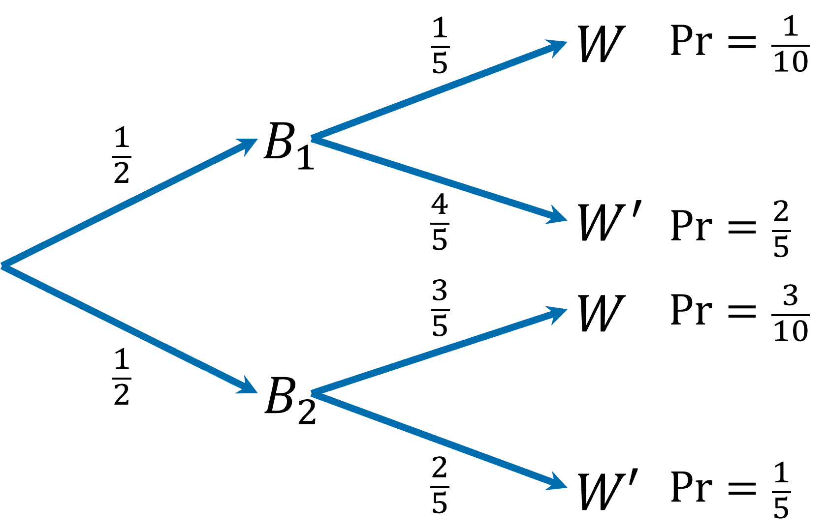
Law of Total Probability
The Law of Total Probability helps you find the overall probability of an event that may occur under different conditions (or within different partitions of the sample space).
A tree diagram is an effective way to represent the sample space of multi-stage or compound events. Probabilities at each stage are calculated by multiplying along the branches, illustrating the multiplication rule of probability.

To determine the probability of a particular event, we sum the probabilities of all outcomes that include that event. This process leads to the Law of Total Probability, which for complementary events can be expressed as:
\(\Pr(B) = \Pr\left(B|A\right)\Pr(A)+\Pr\left(B|A^\prime \right)\Pr(A^\prime)\)
This formula accounts for all possible scenarios that contribute to the occurrence of event \(B\).
Check your understanding
View
Probability Tables
Probability tables are a valuable tool for solving problems involving compound events — situations where two or more different events happen together. These tables help by organizing all the possible outcomes (the sample space) into a clear and structured format, making analysis much simpler.
Each cell shows the probability of a specific outcome combination, and each row or column must sum to its total. By filling in the table, you can, easily find probabilities of combined events, quickly calculate related probabilities and confirm that all probabilities sum to 1.
| \(B\) | \(B^\prime\) | ||
|---|---|---|---|
| \(A\) | \(\Pr\left(A\cap B\right)\) | \(\Pr\left(A\cap B^\prime\right)\) | \( \Pr(A)\) |
| \(A^\prime\) | \(\Pr\left(A^\prime\cap B\right)\) | \(\Pr\left(A^\prime\cap B^\prime\right)\) | \( \Pr(A^\prime)\) |
| \( \Pr(B)\) | \(\Pr(B^\prime) \) | \(\Pr(\varepsilon) \) |
Worked Example
If \(\Pr(A)=0.25\), \(\Pr(B)=0.35\) and \(\Pr(A\cap B)=0.1\), complete a probability table for the compound events \(A\) and \(B\).
Construct the probability table and fill in the known values
| \(B\) | \(B^\prime\) | ||
|---|---|---|---|
| \(A\) | \(0.1\) | \(0.25\) | |
| \(A^\prime\) | |||
| \(0.35\) | \(1\) |
Then, the rest of the table can be completed using the fact that each row and column must sum to its total.
For example, if we know
\( \Pr(A)=\Pr\left(A\cap B\right)+\Pr\left(A\cap B^\prime\right)\)
Then,
\(\Pr\left(A\cap B^\prime\right)=0.25-0.1=0.15\)
| \(B\) | \(B^\prime\) | ||
|---|---|---|---|
| \(A\) | \(0.1\) | \(0.15\) | \(0.25\) |
| \(A^\prime\) | \(0.25\) | \(0.5\) | \(0.75\) |
| \(0.35\) | \(0.65\) | \(1\) |