Graphs of exponential and logarithmic functions
Graphs of Exponential and Logarithmic Functions
Graphs of exponential functions and logarithmic functions provide a visual insight into their properties, such as growth, decay, and the inverse relationship between them. Graphs of exponential functions allow us to examine the distinctive curve of exponential growth and decay, while graphs of logarithmic functions facilitate analysis of the inverse of exponentials.
Use this page to revise the following concepts of graphing exponential and logarithmic functions:
- Graphs of Exponential Functions
- Graphs of Logarithmic Functions
- Transformations of graphs of exponential and logarithmic functions
- Graph transformations of exponential functions
- Graph transformations of logarithmic functions
- Inverse relationship between exponential and logarithmic functions
Graphs of Exponential Functions
An exponential function is a mathematical function in the form of \( f(x) = a^x \) where \(x\) is an exponent and \(a\) is a constant (also known as the base) and where \( a \in \mathbb{R}^+ \setminus \{ 1 \}\). The most commonly used base is the Euler’s number, \(e\), which is approximately equal to \(2.71828\).
Generally, there are two scenarios of exponential functions, exponential growth and exponential decay. Each scenario is modelled by a specific graph.
Exponential growth is modelled by functions of the form \( f(x) = a^x\) where \( a \) is greater than \(1\).
For example, the graph of \( f(x) = 2^x \) is shown below.
| Graph of \( y=f(x) = 2^x \) | Key features of \( y=f(x) = a^x \) where \(a > 1\) |
|---|---|

|
|
NoteThese features hold for the form \( f(x) = a^x \). However, if transformations are applied, the \(y\)-intercept and range will change accordingly. |
Exponential decay is modelled by functions of the \( f(x) = a^x\) where \( a \) is greater than \(0\) but less than \(1\). For example, the graph of \(f(x)=\left(\frac{1}{2}\right)^x\) is shown below and key features are summarised.
| Graph of \( y=f(x) = \left(\frac{1}{2}\right)^x \) | Key features of \( y=f(x) = a^x \) where \(0 < a < 1\) |
|---|---|
 |
|
NoteThese features hold for the form \( f(x) = a^x \). However, if transformations are applied, the \(y\)-intercept and range will change accordingly. Note that \(\left(\frac{1}{a}\right)^x\) is equivalent to \(a^{-x}\). When it is graphed, it can be seen that it is a reflection of \(a^x\) across the \(y\)-axis. |
 Check your understanding
View
Check your understanding
View

Graphs of Logarithmic Functions
The logarithmic function is the inverse function to the exponential function. The logarithmic function is defined as \(f(x) = \log_a(x)\) where \(x \in \mathbb{R}^+\) and \(a \in \mathbb{R} \setminus \{ 1\}\). The base of the logarithm is \(a\), this can be read as "\(\log\) base \(a\) of \(x\)". The most two common bases used in logarithmic functions are base 10 and base \(e\).
The logarithmic function with base \(10\) is called the common logarithmic function and it is denoted by \(f(x) = \log_{10}(x)\).
The logarithmic function with base \(e\) is called the natural logarithmic function and it is denoted by \(f(x) = \log_e(x)\) or \(f(x) = \ln(x)\).
Generally, there are two types of graphs of logarithmic functions of the form \(f(x) = \log_a(x)\), depending on the value of \(a\).
- If \(a > 1\), the graph is going up and passing through \((1,0)\)
- If \(0 < a < 1\), the graph is going down and passing through \((1,0)\)
This behaviour can be changed by transformations, which are discussed later.
- The graph of logarithmic function when 𝑎 \( > 1\)
- The graph of logarithmic function when \(0 < \) 𝑎 \( < 1\)
The logarithmic function (going up) is denoted by \(f(x) = \log_a(x)\) where \( a > 1 \). The graph of \(f(x) = \log_2(x)\) is shown below, and key features summarised.
For example, the graph of \( f(x) = \log_2(x) \) is shown below.
| Graph of \(y=f(x) = \log_2(x)\) | Key features of \(y=f(x) = \log_a(x)\) where \(a > 1\) |
|---|---|

|
|
The logarithmic function (going down) is denoted by \(f(x) = \log_a(x)\) where \( 0 < a < 1 \). The graph of \(f(x) = \log_{\frac{1}{2}}(x)\) is shown below, and key features summarised.
| Graph of \(y=f(x) = \log_{\frac{1}{2}}(x)\) | Key features of \(y=f(x) = \log_a(x)\) where \(0 < a < 1\) |
|---|---|

|
|
Check your understanding
View
Transformations of graphs of exponential and logarithmic functions
Transformations of exponential and logarithmic function graphs involve dilating (also known as stretching or compressing), reflecting, and translating (also known as shifting or moving) to create new versions of the original graphs.
Generally, there are three types of transformations that could be applied to each function.
- Dilations – stretches or compresses
- Reflections – flip the graph
- Translations – shifts or movements
For example:
- Horizontal and vertical shifts move the graph left, right, up or down
- Stretching or compressing alters the steepness or width of a graph
- Reflections flip the graph across an axis, changing its orientation
Graph transformations of exponential functions
Transformations of exponential graphs behave similarly to those of other functions.
Three types of transformations can be applied to the original exponential function given by \(f(x) = \log_a(x)\) where \( a \in \mathbb{R}^+ \setminus \{ 1 \}\).
- Shifts – horizontal and vertical
- Reflections – in the \(x\)-axis and \(y\)-axis
- Stretches/compressions – horizontal and vertical
| Stretches | Compressions |
|---|---|
|
Suppose \(a > 1\), to obtain the graphs of: \[y = m \times f(x) = mx^x\] Stretch the graph of \(y = f(x)\) vertically by a factor of \(m\). For example, to obtain \(y = 3 \times 2^x\) from \(y = 2^x\).  The blue curve represents \(y = 2^x\), and the green represents \(y = 3 \times 2^x\). The original graph of \(y = 2^x \) is now stretching vertically by a factor of \(3\) (triple in \(x-\)values). |
Suppose \(a > 1\), to obtain the graphs of: \[ y = \frac{1}{m} \times f(x) = \frac{1}{m} \times a^x \] Stretch the graph of \(y = f(x)\) vertically by a factor of \(m\). For example, to obtain \(y = \frac{1}{2} \times 2^x \) from \(y = 2^x\).  The blue curve represents \(y = 2^x\), and the green represents \(y = \frac{1}{2} \times 2^x \). The original graph of \(y = 2^x \) is now compressed vertically by a factor of \(2\) (half in \(y-\)values). |
|
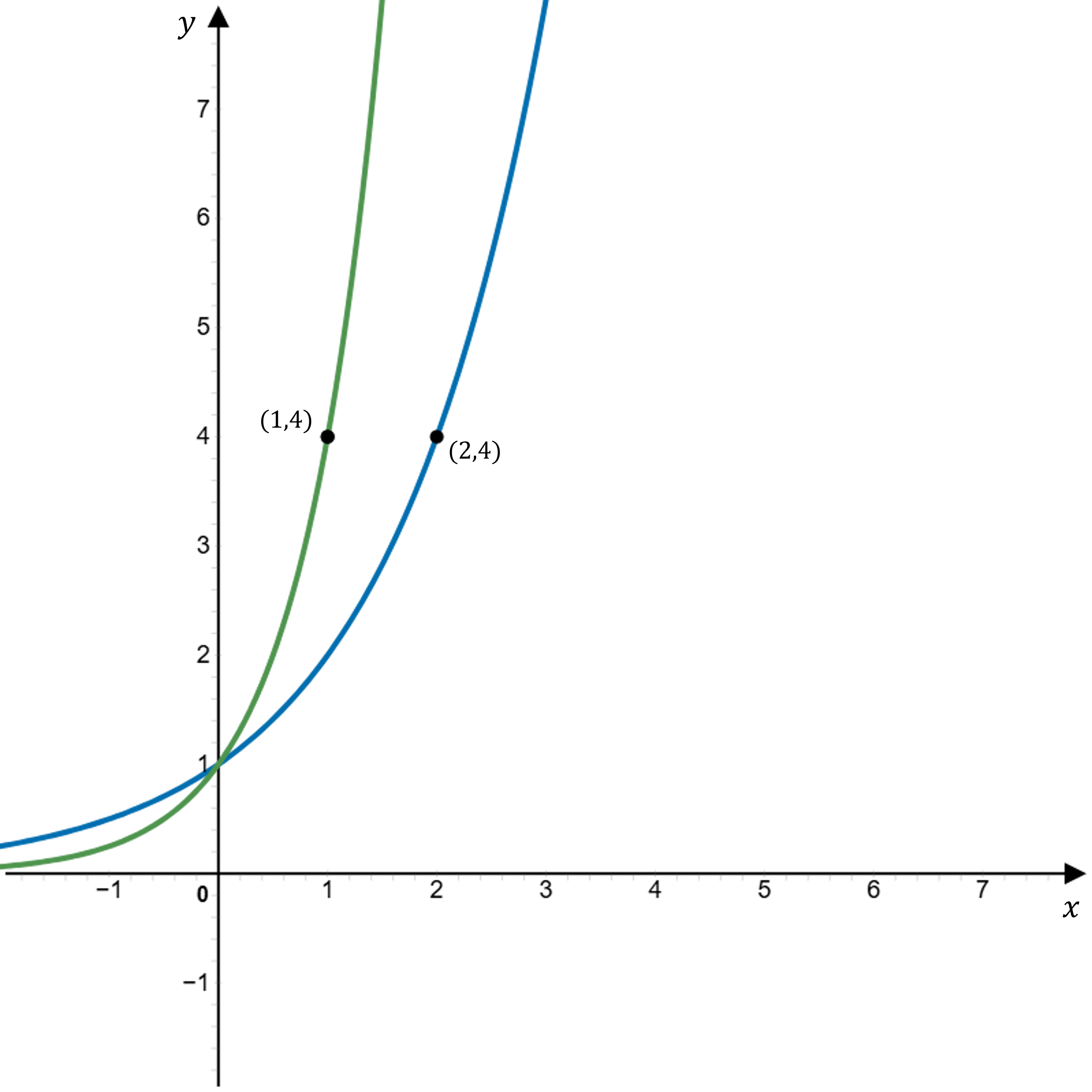
\[ y = f\left(\frac{x}{m}\right) = a^{\left(\frac{x}{m}\right)} \] Stretch the graph of \(y = f(x)\) horizontally by a factor of \(m\). For example, to obtain \( y = 2^{\frac{x}{3}} \) from \(y = 2^x\).  The blue curve represents \(y = 2^x\), and the green represents \( y = 2^{\frac{x}{3}} \). The original graph of \(y = 2^x \) is now stretching horizontally by a factor of \(3\) (triple in \(x\)-values). | \[ y = f(mx) = a^{mx} \]
The blue curve represents \(y = 2^x\), and the green represents \( y = 2^{2x} \). |
| In the \(x\)-axis | In the \(y\)-axis |
|---|---|
| Reflect the graph of \(y = f(x)\) in the \(x\)-axis. \[y=-f(x)=-a^x\] For example, to obtain \(y = -2^x\) from \(y = 2^x\).  The blue curve represents \(y = 2^x\), and the green represents \(y = -2^x\). The original graph of \(y = 2^x \) is now reflected in the \(x\)-axis (flipped upside down). | Reflect the graph of \(y = f(x)\) in the \(x\)-axis. \[y=f(-x)=a^{-x}\] For example, to obtain \(y = -2^x\) from \(y = 2^x\). 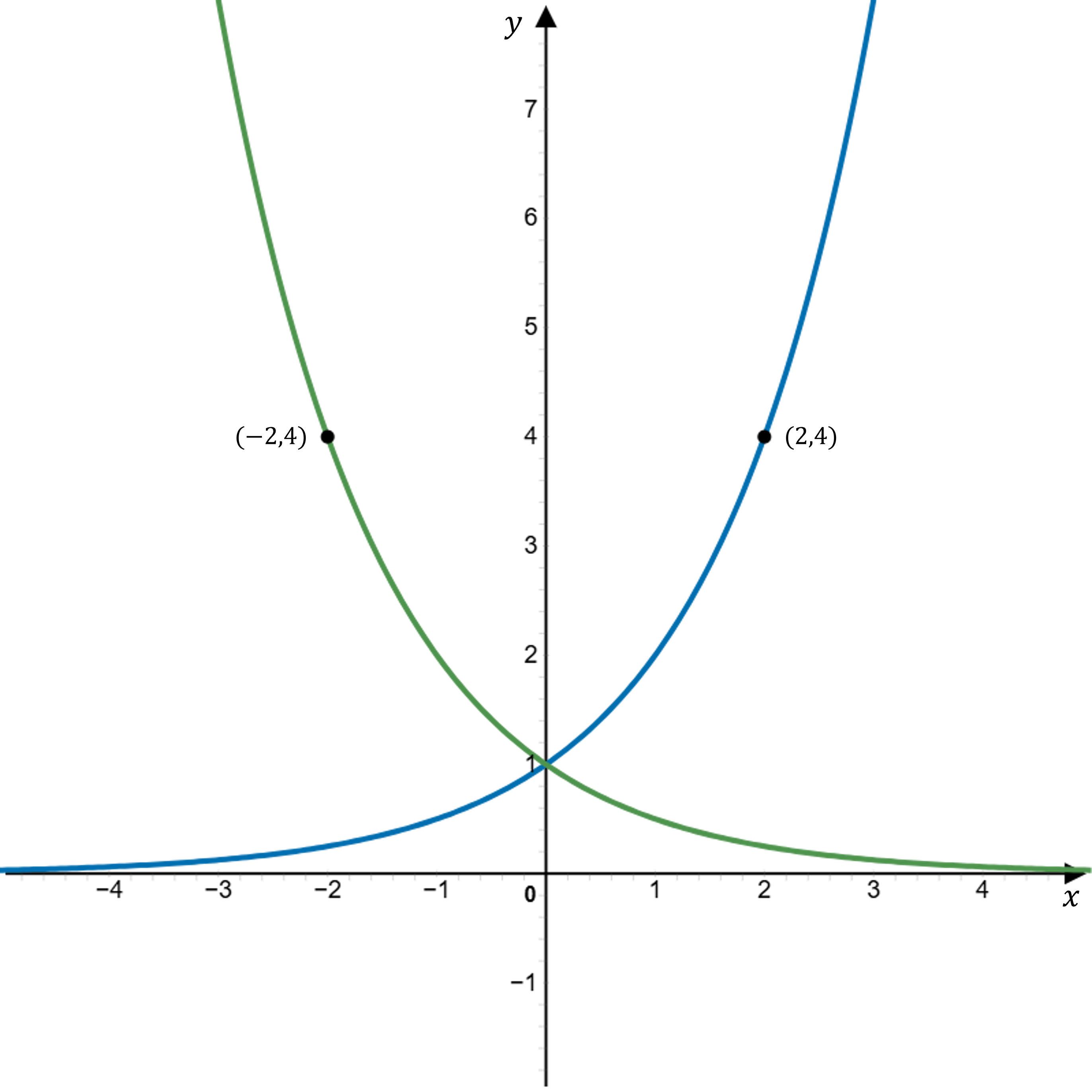 The blue curve represents \(y = 2^x\), and the green represents \(y = 2^{-x}\). The original graph of \(y = 2^x \) is now reflected in the \(y\)-axis. |
| In the \(x\)-axis | In the \(y\)-axis |
|---|---|
| Shift the graph of \(y = f(x)\) to the right by \(h\) units. \[y = f(x - h) = a^{(x-h)} \] For example, to obtain \(y = 2^{(x - 2)} \) from \(y = 2^x\).  The blue curve represents \(y = 2^x\), and the green represents \(y = 2^{(x-2)}\). The original graph of \(y = 2^x \) is now shifted to the right by \(2\) units. | Shift the graph of \(y = f(x)\) up by \(k\) units. \[y = f(x) + k = a^x + k \] For example, to obtain \(y = 2^x + 2 \) from \(y = 2^x\).  The blue curve represents \(y = 2^x\), and the green represents \(y = 2^x + 2\). The original graph of \(y = 2^x \) is now shifted up by \(2\) units. |
| Shift the graph of \(y = f(x)\) to the left by \(h\) units. \[y = f(x - h) = a^{(x-h)} \] For example, to obtain \(y = 2^{(x + 2)} \) from \(y = 2^x\). 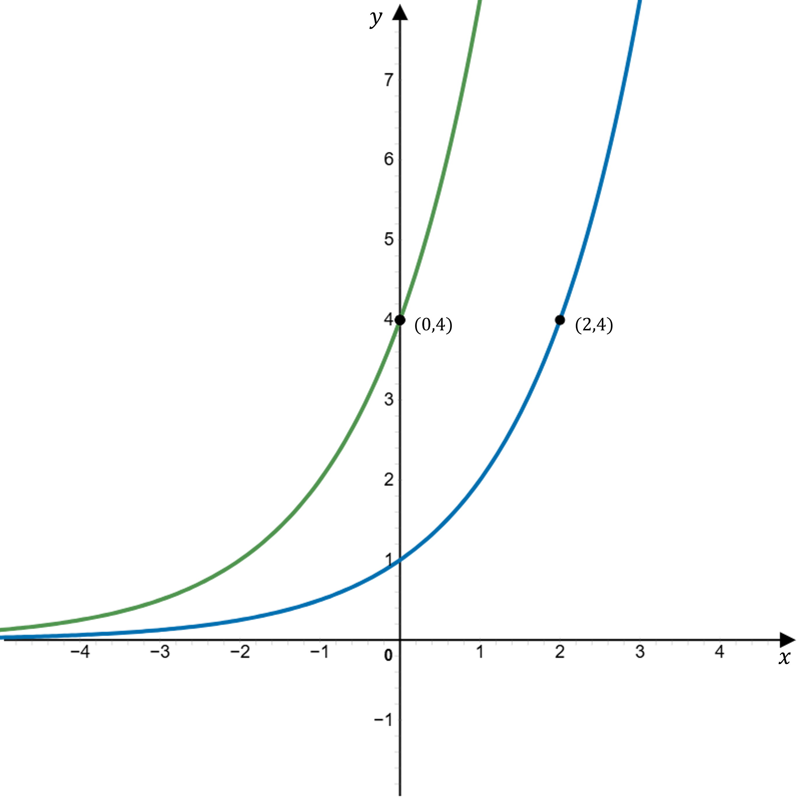 The blue curve represents \(y = 2^x\), and the green represents \(y = 2^{(x+2)}\). The original graph of \(y = 2^x \) is now shifted to the left by \(2\) units. | Shift the graph of \(your = f(x)\) down by \(k\) units. \[y = f(x) - k = a^x - k \] For example, to obtain \(y = 2^x - 2 \) from \(y = 2^x\).  The blue curve represents \(y = 2^x\), and the green represents \(y = 2^x - 2\). The original graph of \(y = 2^x \) is now shifted down by \(2\) units. |
Graph transformations of logarithmic functions
Transformations of logarithmic graphs behave similarly to those of other functions.
Three types of transformations can be applied to the original logarithmic function given by \(f(x) = a^x\) where \(a \in \mathbb{R}^+\) and \(a \neq 1\).
- Shifts – horizontal and vertical
- Reflections – in the \(x\)-axis and \(y\)-axis
- Stretches/compressions – horizontal and vertical
| Stretches | Compressions |
|---|---|
Suppose \(a > 1\), to obtain the graphs of:
The blue curve represents \(y = \log_{2}(x)\), and the green represents \(y = 3 \times \log_{2}(x)\). | Suppose \(a > 1\), to obtain the graphs of:
The blue curve represents \(y = \log_{2}(x)\), and the green represents \( y = \frac{1}{2} \times \log_2(x) \). |
Stretch the graph of \(y = f(x)\) horizontally by a factor of \(m\).\[ y = f\left(\frac{x}{m}\right) = \log_a\left(\frac{x}{m}\right) \]
The blue curve represents \(y = \log_{2}(x)\), and the green represents \( | Compress the graph of \(y = f(x)\) horizontally by a factor of \(m\).\[y = f(mx) = \log_{a}(mx)\]
The blue curve represents \(y = \log_{2}(x)\), and the green represents \(y = \log_{2}(2x)\). |


| In the \(x\)-axis | In the \(y\)-axis |
|---|---|
| Reflect the graph of \(y= f(x)\) in the \(x\)-axis. \[y=-f(x)=-\log_{a}(x)\] For example, to obtain \(y = -\log_{2}(x)\) from \(y = \log_{2}(x)\).
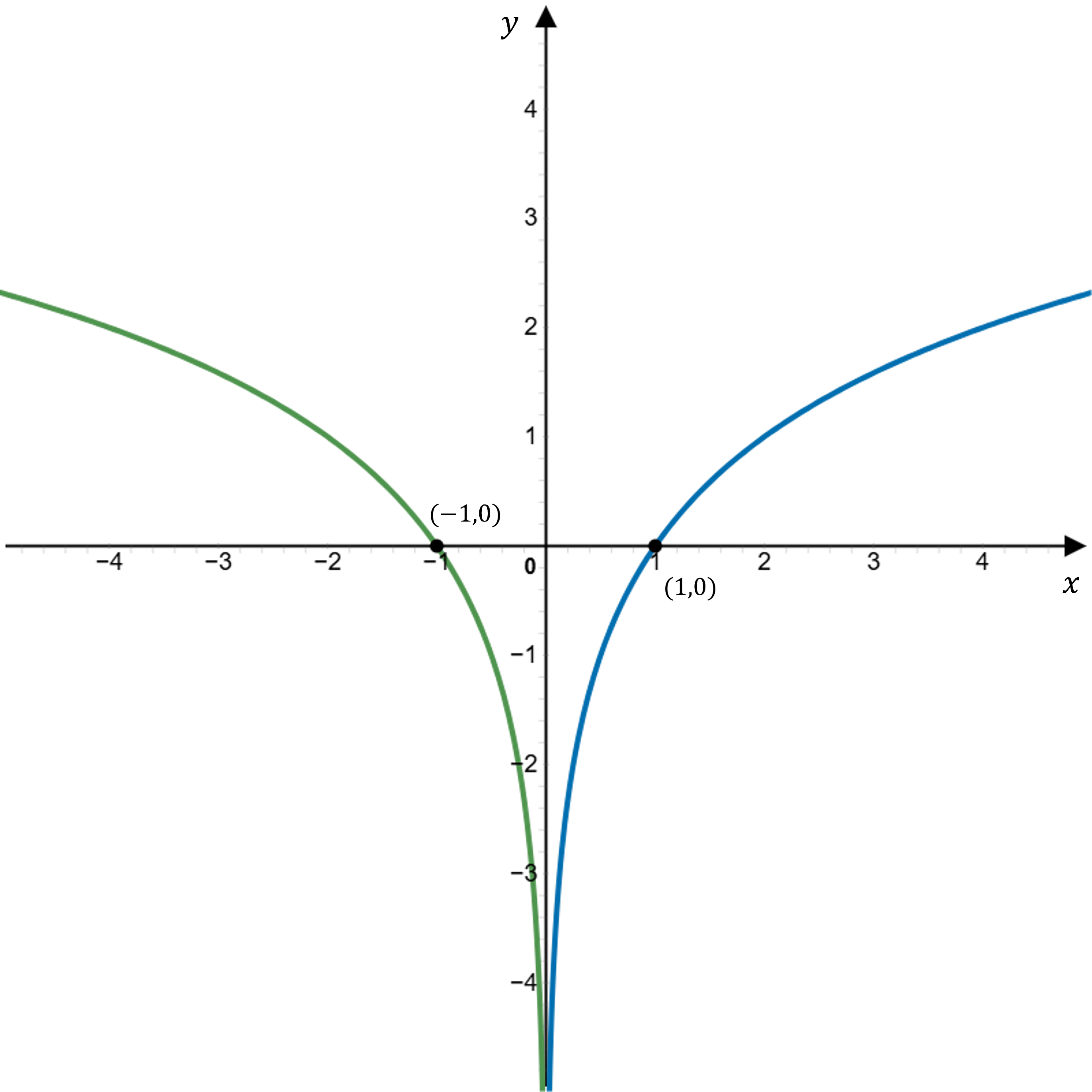
| Reflect the graph of \(y = f(x)\) in the \(y\)-axis. \[y=f(-x)=\log_{a}(-x)\] For example, to obtain \(y = \log_{2}(-x)\) from \(y = \log_{2}(x)\).
The original graph of \(y = \log_{2}(x)\) is now reflected in the \(y\)-axis. |

| Horizontal shifts | Vertical shifts |
|---|---|
|
Shift the graph of \(y = f(x)\) to the right by \(h\) units. \[ y = f(x - h) = \log_a(x - h) \] For example, to obtain \(y = \log_2(x - 2) \) from \(y = \log_2(x)\).  The blue curve represents \(y = \log_2(x) \), and the green represents \(y = \log_2(x-2) \). The original graph of \(y = \log_2(x) \) is now shifted to the right by \(2\) units. |
Shift the graph of \(y = f(x)\) up by \(h\) units. \[ y = f(x) + k = \log_a(x) + k \] For example, to obtain \(y = \log_2(x) + 2 \) from \(y = \log_2(x)\). 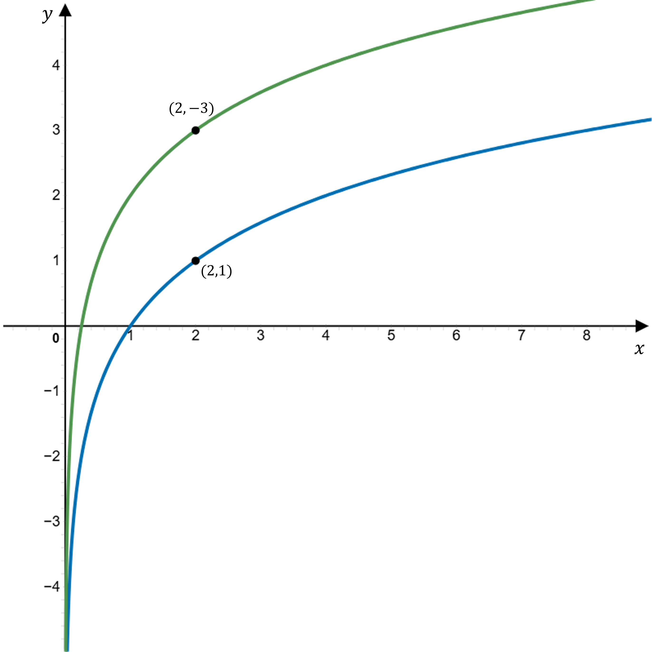 The blue curve represents \(y = \log_2(x) \), and the green one represents \(y = \log_2(x) + 2 \). The original graph of \(y = \log_2(x) \) is now shifted up by \(2\) units. |
|
Shift the graph of \(y = f(x)\) to the left by \(h\) units. \[ y = f(x + h) = \log_a(x + h) \] For example, to obtain \(y = \log_2(x + 2) \) from \(y = \log_2(x)\).  The blue curve represents \(y = \log_2(x) \), and the green represents \(y = \log_2(x+2) \). The original graph of \(y = \log_2(x) \) is now shifted to the left by \(2\) units. |
Shift the graph of \(y= f(x)\) down by \(k\) units. \[ y = f(x) - k = \log_a(x) - k \] For example, to obtain \(y = \log_2(x) - 2 \) from \(y = \log_2(x)\).  The blue curve represents \(y = \log_2(x) \), and the green represents \(y = \log_2(x) - 2 \). The original graph of \(y = \log_2(x) \) is now shifted down by \(2\) units. |
Check your understanding
View
Inverse relationship between exponential and logarithmic functions
The exponential function and the logarithmic function are inverses of each other, meaning they ‘undo’ each other’s operations.
If the exponential function is given by \(f(x) = a^x\) where \( a \in \mathbb{R}^+ \setminus \{1\} \), then its inverse is the logarithmic function \(g(x) = \log_{a}(x)\) where \( a \in \mathbb{R}^+ \setminus \{ 1 \}\). This relationship implies that applying the logarithmic function to the result of an exponential function returns the original input, and vice versa.
For example, if \(y = a^x\), then taking \(\log_{a}(y)\) yields \(x\), because \(\log_{a}(a^x) = x\). Similarly, if \(y = \log_{a}(x)\), then \( a^y = a^{\log_{a}(x)} = x \).
This inverse relationship is a fundamental property that links these two functions and forms the basis for solving equations involving exponential growth or decay and their corresponding logarithmic expressions.
Properties of inverses
| Explanation using graph | Summary of properties |
|---|---|
|
|
