Cubics and quartics
Cubic and quartic functions are the natural extension of polynomials after quadratics, representing higher-order polynomials with degrees three and four respectively.
A cubic function can be expressed as:
\[f(x) = a_3x^3 + a_2x^2 + a_1x + a_0\]
A quartic function can be expressed as:
\[f(x) = a_4x^4 + a_3x^3 + a_2x^2 + a_1x + a_0\]
Understanding these polynomials provides the foundation for comprehending all polynomials, as they share many features that can be generalised to higher orders. This understanding is rooted in recognising the nature of the polynomial's degree, whether odd or even. As a result, it offers an endless variety of polynomials that can be applied flexibly to model real-world scenarios which are often more complex.
Use this page to revise the following concepts of cubic and quartic functions:
- Solving Cubic and Quartic Equations
- Graphing Cubic and Quartic Functions
- Transformation of Cubic and Quartic Functions
Solving Cubic and Quartic Equations
Solving cubic and quartic equations can be more challenging due to their higher order, which makes finding the appropriate factors for factorisation more difficult. However, there are various strategies that can be used to simplify the process. By combining these strategies with those used for quadratic equations, the solutions for cubic and quartic equations can be determined.
Factor and Remainder Theorems
The factor theorem provides a simple way of determining whether a given value is a factor of a polynomial, while the remainder theorem offers a method to calculate the remainder when a polynomial is divided by a linear divisor.
By substituting a value into a polynomial, \(f(a)\), if:
- The result of \(f\left(a\right) = 0\), then \(\left(x - a\right)\) is a factor of the polynomial \(f\left(x\right)\)
- The result of \(f(a)\) is other than 0, then if \(f(x)\) were to be divided by \((x - a)\) it would result in a remainder of \(f(a)\).
Worked Example
Consider the function:
\[f(x) = x^3 - 4x^2 + x +6\]
Values for \(x\) can be substituted to determine whether they are factors using the Factor Theorem and Remainder Theorem.
For \(x =1\),
\[f(1) = (1)^3 - 4(1)^2 + (1) + 6 = 4\]
Since \(f(1) = 4\):
- Factor theorem: \(\left(x - 1\right)\) is not a factor of \(x^3 - 4x^2 + x + 6\)
- Remainder theorem: If \(x^3 - 4x^2 + x + 6\) is divided by \((x - 1)\), the remainder would be 4.
For \(x=2\),
\[f(2)=(2)^3-4(2)^2+2+6=0\]
Since \(f\left(2\right) = 0\):
- Factor theorem: \(\left(x - 2\right)\) is a factor of \(x^3 - 4x^2+ x + 6\)
- Remainder theorem: If \(x^3 - 4x^2+ x + 6\) is divided by \((x - 2)\), there would be no remainder, confirming that it is a factor.
Factorising fully:
\[\begin{align} f(x)&=(x-2)(x^2-2x-3)\\ &=(x-2)(x-3)(x+1) \end{align}\]
Check your understanding
View

Rational Root Theorem
Substituting random values for \(x\) to determine factors of a polynomial can be inefficient, especially for more complex polynomials. The Rational Root Theorem provides a systematic way of narrowing down potential factors or solutions based on the polynomial's leading coefficient and constant term.
For a polynomial:
\[f(x) = a_nx^n + a_{n-1}x^{n-1} + \cdots + a_1x + a_0\]
The theorem states that it must have rational roots in the form of \(\dfrac{p}{q}\)
- \(p\) must be a factor of \(a_0\)
- \(q\) must be a factor of \(a_n\)
This greatly reduces the number of potential roots to test to factorise a polynomial.
To determine all the potential roots:
- List all the factors of \(a_0\)
- List all the factors of \(a_n\)
- Write down all possible roots \(\dfrac{p}{q}\)
- Consider all unique roots
\[\text{Possible roots} = \pm\frac{\text{factors of }a_0}{\text{factors of }a_n}\]
Worked Example
Consider the function:
\[f(x) = 2x^{3} - 2x^{2} + 8x +8\]
1. Factors of \(a_0\) (constant):
\[\{1, 2, 4, 8\}\]
2. Factors of \(a_n\) (leading coefficient):
\[\{1, 2\}\]
3. Possible roots:
\[\pm\frac{\text{factors of} a_{0}}{\text{factors of} a_{n}}\]
These are all the possible factors without simplifying the fractions:
\[\pm\frac{1}{1}, \pm\frac{2}{1}, \pm\frac{4}{1}, \pm\frac{8}{1}, \pm\frac{1}{2}, \pm\frac{2}{2}, \pm\frac{4}{2}, \pm\frac{8}{2}\]
Once simplified:
\[\pm1, \pm2, \pm4, \pm8, \pm\frac{1}{2}, \pm1, \pm2, \pm4\]
4. Unique roots:
Removing the repetition, the following roots remain:
\[\pm1,\pm2,\pm4,\pm8,\pm\frac{1}{2}\]
There are 10 possible roots to test for \(f\left(x\right) = 2x^3 - 2x^2 + 8x + 8\)
Check your understanding
View
Polynomial Division
Once a single factor is identified, polynomial division can be used to start factorising the polynomial. This method is similar to long division, but instead of aligning digits, terms are aligned by their powers of \(x\). The divisor and quotient represent parts of the polynomial in its factorised form.
The steps for polynomial division are as follows:
- Divide the leading term by the leading term of the divisor to obtain the first term of the quotient
- Multiply this term by the entire divisor
- Subtract the resulting expression from the dividend
- Repeat the process with the newly formed polynomial until the degree of the remainder is less than the degree of the divisor
Worked Example
Consider the function:
\[f(x) =x^{3} -4x^{2} +x +6\]
\(\left(x- 2\right)\) is a known factor:
- Divide the leading term \(\dfrac{x^{3}}{x} = x^{2}\)
- Multiply \(x^{2}\) by the divisor \(\left(x - 2\right)\)
- Subtract the result from the dividend
- Repeat until the quotient is found
\[\begin{align} &x^2 \\ x - 2\big| & \overline{x^3 - 4x^2 + x + 6} \end{align}\]
\[\begin{align}&x^{2}& \\ x - 2&\big|\overline{x^{3} - 4x^{2} + x +6} \\ &x^{3} - 2x^{2}\end{align}\]
\[
\begin{array}{r@{}l}
& \phantom{\big|} x^2 - 2x - 3 \\
x - 2 & \big| \overline{x^3 - 4x^2 + x + 6} \\
& \phantom{\big|} \underline{x^3 - 2x^2} \\
& \phantom{\big|} \phantom{x^3} \smash{-2x^2 + x + 6} \\
\end{array}
\]
\[
\begin{array}{r@{}l}
& \phantom{\big|} x^2 - 2x - 3 \\
x - 2 & \big| \overline{x^3 - 4x^2 + x + 6} \\
& \phantom{\big|} \underline{x^3 - 2x^2} \\
& \phantom{\big|} \phantom{x^3} \smash{-2x^2 + x + 6} \\
& \phantom{\big|} \phantom{x^3} \underline{-2x^2 + 4x} \\
& \phantom{\big|} \phantom{x^3-2x^2} \smash{-3x + 6} \\
& \phantom{\big|} \phantom{x^3-2x^2} \underline{-3x + 6} \\
& \phantom{\big|} \phantom{x^3-2x^2-3x +} \smash{0} \\
\end{array}
\]
Therefore, the function can be expressed as:
\[\begin{align}f(x) &= x^{3} -4^{2} + x + 6 \\ &= (x - 2)(x^{2} - 2x - 3)\end{align}\]
Polynomial division can also be performed when there is a remainder. In such cases, the remainder can be written as a term divided by the divisor, forming a rational expression.
Worked Example
Consider the function:
\[f(x) = x^{3} - 4x^{2} + x+ 6\]
As \(f\left(1\right)=4\), the rational root theorem states that there is a remainder of 4 when the function is divided by \((x - 1)\)
Dividing \(f(x)\) by \(\left(x - 1\right)\) results in the quotient
\[x^{2} - 3x - 2\]
Since there is a remainder of 4, the function can be expressed as:
\[\begin{align}f(x) &= x^{3} - 4x^{2} + x +6 \\ &= (x - 1)(x^{2} - 3x -2) +4\end{align}\]
Alternatively, it can also be written as:
\[f(x) = \left(x - 1\right)\left(x^{2} - 3x - 2 + \frac{4}{x - 1}\right)\]
Check your understanding
View
Graphing Cubic and Quartic Functions
The shape of cubic and quartic functions varies, but they share some key features. These include:
- \(x\)- and \(y\) -intercepts: The points where the graph crosses the axes.
- Stationary points: The points on the graph where the slope (or gradient) is zero.
- End points (if applicable): The boundaries of the graph when the domain is restricted. This is the determined similarly for other functions, by substituting the ends of the domains into the function.
Shape of Cubic Functions
Cubic functions are typically represented by an S-shaped graph, however the specific rise and fall of the graph depend on equation. They may exhibit a stationary point of inflection, a non-stationary point of inflection, or two distinct turning points (local minimum and local maximum, which are not symmetrical.
The basic cubic function \(f(x) = x^{3}\) is graphed below:

The direction of the graph depends on the leading coefficient in the function:
\[f(x) = ax^{3} + bx^{2} + cx +d\]
- If \(a > 0\): The graph extends from negative infinity (bottom left) to positive infinity (top right)
- If \(a < 0\): The graph extends from positive infinity (top left) to negative infinity (bottom right)
A cubic function can take one of three primary shapes, defined by a specific feature:
- A Stationary Point of Inflection:
- A Non-Stationary Point of Inflection:
- Two Distinct Turning Points:
This occurs when the cubic function is a perfect cube.
\[f(x) = a\left(b\left(x- c\right)\right)^{3} +d\]
The stationary point of inflection is the point where the slope tapers to zero, resulting in a horizontally flat slope, before increasing in the same direction again. This is pictured in the graph above.
This is where the slope of the graph gradually decreases to a minimum value, and then increase in the same direction again smoothly without ever reaching a point with zero slope.

These are points on the graph where the slope is zero, indicating a change in direction. Unlike some other functions, the graph of a cubic function is not symmetrical around these points.
Nature of Turning Points:
- Local Minimum: Slope changes from negative (downwards) to positive (upwards)
- Local Maximum: Slope changes from positive (upwards) to negative (downwards)
The coordinates of these points can only be determined using calculus – finding the \(x\)-coordinate of the turning point when \(f^\prime\left(x\right) = 0\).

Shape of Quartic Functions
Quartic functions are typically represented by a U-shaped graph like parabolas.
The basic quartic function \(f(x) = x^4\) is graphed below:

However, depending on the equation, quartic functions may also resemble a W-shaped graph, where the shape between the two ends varies significantly:
- Example of a quartic function with three turning points
- Example of a quartic function with one turning point and one stationary point of inflection:


The direction of the graph depends on the leading coefficient in the function:
\[f(x) = ax^{4} + bx^{3} + cx^{2} + dx + e\]
- If \(a > 0\): The graph starts from positive infinity (top left), turns around and then returns to positive infinity (top right)
- if \(a < 0\): The graph starts from negative infinity (bottom left), turns around and then returns to negative infinity (bottom right)
Stationary Points
The stationary points of more complex cubic, quartic and higher order polynomial functions can be determined using calculus, as their graphs around these points are not typically symmetrical.
The derivative of the function describes the slope of the graph. Stationary points occur where the slope is zero, meaning the derivative equals zero. To determine the coordinates of the stationary points:
- Sovle for \(x\), where \(f^\prime\left(x\right) = 0\)
- Substitute \(x\) values into \(f\left(x\right)\) to find the corresponding coordinates
Axial Intercepts
The key to determining the shape of a cubic or quartic graph lies in identifying the \(x\)- and \(y\)- intercepts. These points combined with the direction given by the leading coefficient provides the overall structure of the graph.
The axial intercepts are the points where the graphs cross the axes. These are also known as the solutions or roots of the equation. Since there are two axes, there are two types of axial intercepts:
- The \(x\)-intercept: the point(s) where the graph crosses the \(x\)-axis
- The \(y\)-intercept: the point where the graph crosses the \(y\)-axis
The \(x\)-axis corresponds to the horizontal line \(y = 0\); and the \(y\)-axis corresponds to the vertical line \(x = 0\). As they correspond to these values, these can be substituted into the function to determine the \(x\)- and \(y\)-intercepts.
The key difference between cubic and quartic functions compared to quadratic functions is in the behaviour of the graph at the \(x\)-intercepts. This behaviour, also known as the nature of the \(x\)-intercepts, depends on the types of factors present in the equation and is only relevant when the equation can be factorised.
The nature of the \(x\)-intercepts are as follows:
Factors in the form of \(\left(x-b\right)\)
Graph passes through the \(x\)-intercept:

Factors in the form of \(\left(x-c\right)^2\)
Graph has a turning point at the \(x\)-intercept:
Factors in the form of \(\left(x-d\right)^3\)
Graph has a point of inflection at the \(x\)-intercept:

Higher-order factors can also be considered, but their behaviour at the \(x\)-intercepts depends on whether the degree is odd or even. As the degree of the factor increases, it produces a flatter effect near the intercept without fundamentally altering the nature of the graph’s interaction with the axis.
- Even Degree Factors:
- Turning point at the \(x\)-intercept
- The curve of the graph is flatter near the stationary point as the degree increases
- Odd Degree Factors:
- Stationary point of inflection at the \(x\)-intercept
- The curve of the graph is flatter near the stationary point as the degree increases
Worked Example
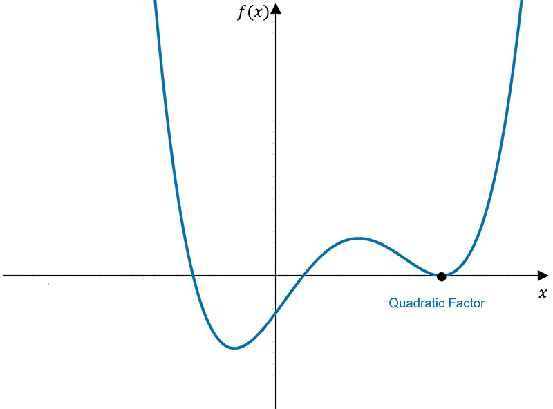
Sketch a graph of the function:
\[f(x) = -\left(x + 2\right)^{2}\left(x - 1\right)\left(x - 3\right)\]
The leading coefficient is negative \(a < 0\), therefore the quartic begins in the bottom left and ends at the bottom right.
The \(y\)-intercept can be calculated:
\[f(0) = -\left(2\right)^{2}\left(-1\right)\left(-3\right) = -12\]
The \(x\)-intercepts can be derived from the factored form.
- \(\left(x - 2\right)^2\) is a quadratic factor at \(x = 2\)
- \(\left(x - 1\right)\) is a linear factor at \(x = 1\)
- \(\left(x - 3\right)\) is a linear factor at \(x = 3\)
Other stationary points can be determined using calculus:
\(f^\prime(x) = 0\)
\(x = 1\pm\frac{\sqrt{6}}{2}\)
Stationary points at: \(\left(1 - \dfrac{\sqrt{6}}{2},\dfrac{9}{4} - 6\sqrt{6}\right)\) and \(\left(1 + \dfrac{\sqrt{6}}{2},\dfrac{9}{4} + \sqrt{6}\right)\)
These points are summarised in the image below:
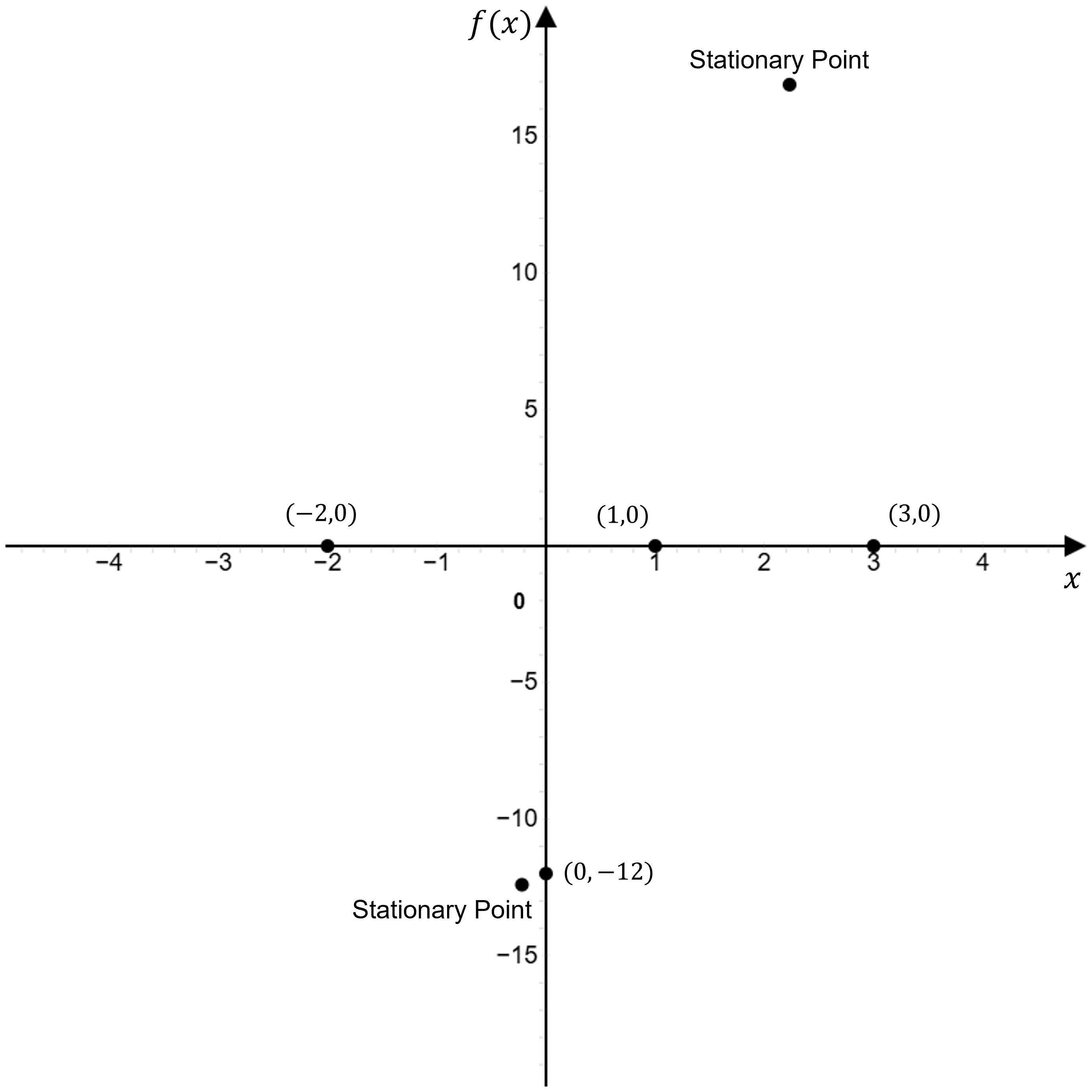
Connecting these points, we can draw the graph of the function:

Check your understanding
View
Transformation of Cubic and Quartic Functions
Transformations of cubic and quartic functions can be easily identified when they are in the following forms:
- Cubic function
- Quartic function:
\[f(x) = a\left(b\left(x - c\right)\right)^{3} +d\]
\[f(x) = a\left(b\left(x - c\right)\right)^{4} + d\]
In both functions, the transformation factors correspond to the following characteristics:
Dilation from the x-axis and reflection in the \(x\)-axis \((a)\)
- Determines the vertical dilation by a factor of \(a\)
- If \(a < 0\), there is also a reflection in the \(x\)-axis
Dilation from the y-axis and reflection in the \(y\)-axis \((b)\)
- Determine the horizontal dilation by a factor of \(\dfrac{1}{b}\)
- If \(b < 0\), there is also a reflection in the \(y\)-axis
- For cubic functions (odd degree): The reflection is visible and results in the graph flipping horizontally.
- For quartic functions (even degree): The reflection does not affect the appearance of the graph, as it is symmetrical about the \(y\)-axis.


- Horizontal translation \((c)\), if:
- \(c > 0\), translation of \(c\) units in the positive direction of the \(x\)-axis (the graph shifts \(c\) units to the right)
- \(c < 0\), translation of \(c\) units in the negative direction of the \(x\)-axis (the graph shifts \(c\) units to the left)
- Vertical translation \((d)\), if:
- \(d > 0\), translation of \(d\) units in the positive direction of the \(y\)-axis (the graph shifts \(d\) units upwards)
- \(d < 0\), translation of \(d\) units in the negative direction of the \(y\)-axis (the graph shifts \(d\) units downwards)
The standard form of cubic, quartic, and other polynomial functions can reveal some key transformation factors, though not as comprehensively as other forms.
For the general polynomial:
\[P(x) = a_{n}x^{n} + a_{n - 1}x^{n - 1} + \cdots + a_{1}x + a_{0}\]
- \(a_n = a\): Represents vertical dilation (stretch or compression) and vertical reflection (if negative)
- \(a_0 = d\): Represents the vertical translation (shifting up or down)