Correlation and least squares regression line
Understanding the linear relationship between two numerical variables is essential for effective data analysis. Pearson’s correlation coefficient (\(r\)) measures the strength and direction of an association, while the least squares regression line provides a linear model to describe the relationship and make predictions. Analysing these measures helps in making informed decisions across various fields in real life.
Use this page to revise the following concepts within correlation and least squares regression line :
Pearson’s Correlation Coefficient (\(r\))
Pearson’s correlation coefficient \((r)\) is a numerical measure of how closely data points in the scatterplot tend to cluster around a straight line. \(r\) indicates the strength and direction of a linear relationship between two numerical variables.
It has a value between \(-1\) to \(+1 \left(-1 \leq r \leq1\right)\).
- Positive \(r\) indicates a positive direction of the linear association.
- Negative \(r\) indicates a negative direction of the linear association.
- \(r\) is close to zero indicates weak or no association.
- \(r\) is close to \(-1\) or \(+1\) indicates strong linear associations.
Calculating Pearson’s Correlation Coefficient
Pearson’s correlation coefficient, \(r\), is given by:
\[r = \frac{\Sigma\left(x - \overline{x}\right)\left(y - \overline{y}\right)}{\left(n - 1\right)s_{x}s_{y}}\]
Where:
- \(n\) is the number of pairs of data in the set
- \(s_{x}\) is the standard deviation of the \(x\)-values
- \(s_y\) is the standard deviation of the \(y\)-values,
- \(\overline{x}\) is the mean of the \(x\)-values,
- \(\overline{y}\) is the mean of the \(x\)-values.
However, a calculator or statistical software is typically used to evaluate the value of \(r\).
Assumptions of using Pearson’s Correlation Coefficient
In order to accurately interpret the value of \(r\) as a measure of the strength of an association, there are three key assumptions:
- Both variables are numerical.
- The association is linear.
- There are no outliers in the data. (Similar to the mean and the standard deviation, \(r\) can be affected by outliers, potentially leading to a misrepresentation of the strength of the linear association.)
Note that a correlation shows the strength of the association between two variables, but it does not explain causation. For example, a strong correlation means that two variables tend to change together, however, it does not imply that changing one will cause the other to change.
Classification of the Strength of a Linear Association
| Values | Strength and Direction of the Linear Association |
|---|---|
| \(r = \pm1\) | Perfect positive/negative |
| \(0.75 \leq r < 1\) or \(-1 < r \leq -0.75\) | Strong positive/negative |
| \(0.5 \leq r < 0.75\) or \(-0.75 < 5 \leq -0.5\) | Moderate positive/negative |
| \(0.25 \leq r < 0.5\) or \(-0.5 < r \leq -0.25\) | Weak positive/negative |
| \(-0.25 < r < 0.25\) | No association |
Scatterplot Examples of Pearson’s Correlation Coefficient
| Perfect Negative | Strong negative | Non association | Strong Positive | Perfect positive |
|---|---|---|---|---|
| ||||

 Check your understanding
View
Check your understanding
View

Least Squares Regression Line
Linear regression is the process of modelling an association between two variables using a straight line, known as the regression line. When a regression line (not necessarily a least squares regression line) is drawn, the vertical distance between each point and the regression line is measured, these distances are called residuals. The least squares regression line is the line that minimises the sum of the squared residuals.
Assumptions of Fitting a Least Squares Line to Data
There are three key assumptions, which are the same as those for using Pearson’s correlation coefficient (\(r\)):
- Both variables are numerical.
- The association is linear.
- There are no outliers in the data.
The Equation of the Least Squares Regression Line
The equation of the least squares regression line is given by
\[y = a + bx\]
Where \(a\) is the \(y\)-intercept, and \(b\) is the gradient/slope
The equation of the gradient/slope is given by
\[b = r \times \frac{s_y}{s_x}\]
Where:
- \(r\) is Pearson’s correlation coefficient
- \(s_x\) is the standard deviation of the \(x\)-values
- \(s_y\) is the standard deviation of the \(y\)-values
The equation of the \(y\)-intercept is given by
\[a = \overline{y} - b \times \overline{x}\]
Where
- \(\overline{x}\) is the mean of the \(x\)-values,
- \(\overline{y}\) is the mean of the \(y\)-values.
Note that if the explanatory variable (\(x\)-variable) and the response variable (\(y\)-variable) are not correctly identified before calculating the least squares regression line equation, the result will be incorrect.
Worked Example
For a set of bivariate data that involves the variables, height (\(x\)) and weight (\(y\)), with \(y\) as the response variable, \(r = 0.7591\), \(\overline{x} = 162.2\), \(\overline{y}=55.34\), \(s_x = 6.333\), and \(s_y = 6.483\). Calculate the values of the slope and intercept, rounded to two decimal places, thus determine the equation of the least squares regression line.
Slope
\[\begin{align}b &= r \times \frac{s_y}{s_x} \\ &= 0.7591 \times \frac{6.483}{6.333} \\ &= 0.78 \textsf{(rounded to two decimal places)}\end{align}\]
Intercept
\[\begin{align}a &= \overline{y} - b \times \overline{x} \\ &= 55.34 - \left(0.7591 \times\frac{6.483}{6.333}\right) \times 162.2 \\ &= -70.70 \end{align}\]
Equation of the least squares regression line:
\[y= -70.70 + 0.78x\]
or
\[\text{weight} = -70.70 + 0.78 \times \text{height}\]
Check your understanding
View
Make Predictions Using the Regression Line
Once the equation of the least squares regression line is determined, it can be used to make predictions. However, it should generally be made within the range of data used to generate it.
For the equation of the regression line \(y = a + bx\):
- the slope (\(b\)) represents the average change in the response variable (\(y\)) for every one-unit increase or decrease in the explanatory variable (\(x\)).
- the intercept (\(a\)) represents the average value of the response variable (\(y\)) when the explanatory variable (\(x\)) is \(0\).
- Note that if \(x = 0\) falls outside the observed data range, the intercept (\(a\)) may not have a meaningful interpretation.
Worked Example
A least squares line is to be fitted to the data with the aim of predicting evening congestion level from morning congestion level. The equation of this line is:
\[\text{Evening congestion level} = 10.01 + 0.855 \times \text{morning congestion level}\]
Interpret the slope and the intercept of the regression line in terms of the variables evening congestion level and morning congestion level.
The slope predicts that on average, the evening congestion level increases by 0.835 for every additional unit of morning congestion level. The intercept predicts that, on average, the evening congestion level is 10.01 when there is no morning congestion at all.
Interpolation and Extrapolation
Interpolation occurs when predictions are made within the range of values of the explanatory variable (\(x\)), which is generally considered a reliable method for making predictions.
Extrapolation occurs when predictions are made beyond the observed range of the explanatory variable (\(x\)). Extrapolation should be approached with caution, as the relationship between variables may not hold outside the data range. It is generally considered to be unreliable for making predictions.
Worked Example
The data below shows the study times (in hours) of 9 students and the marks they obtained on a test.
| Time (hours | 6 | 8 | 10 | 11 | 13 | 16 | 18 | 27 | 35 |
|---|---|---|---|---|---|---|---|---|---|
| Mark (%) | 25 | 31 | 32 | 29 | 30 | 40 | 47 | 68 | 82 |
The corresponding scatterplot is shown below.
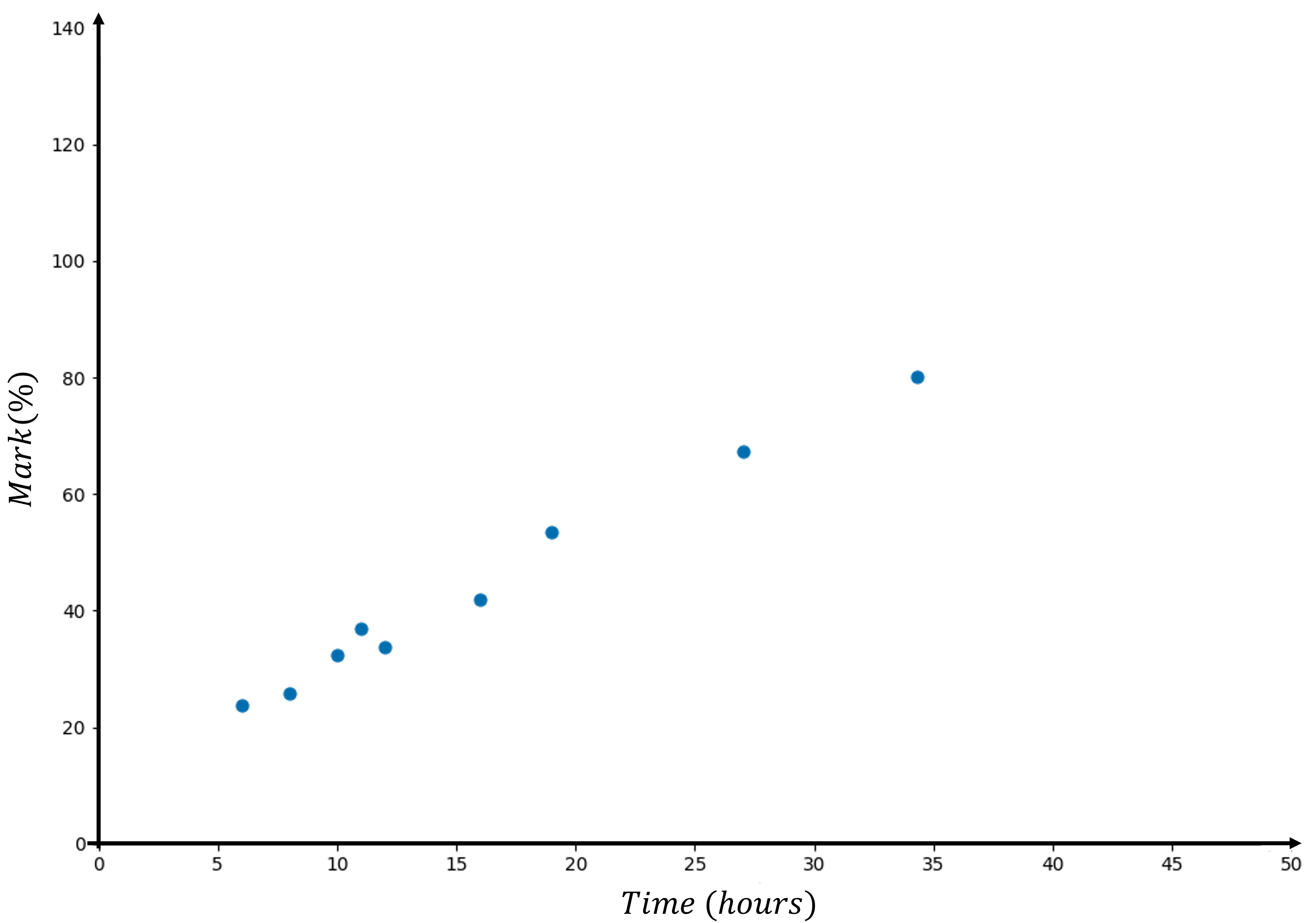
A least squares regression line is used to model the association between the time spent studying (in hours) and the test marks (%) for this group of students, the equation is close to:
\[\text{mark} = 9.889 + 2.045\ \text{time}\]