Fundamental theorem of calculus and the definite integral
The definite integral allows us to accurately calculate the area under a curve. It draws on the concepts of the indefinite integral and estimating the area under the curve. These ideas are combined, allowing the exact area to be calculated rather than approximated.
Use this page to revise the following concepts:
The definite integral
Recall that an indefinite integral (or antiderivative) is so called as it provides a family of solutions with a constant term . It is called indefinite as the constant \(c\) can take any real value, \(c \in \mathbb{R}\).
For example, \(\int2x dx = x^{2} + c\).
In comparison, the definite integral has limits of integration in the integral sign, and finds the difference between the values of the antiderivative at these limits. As a result, the, constant \(c\) becomes redundant, as the definite integrals compute the difference between the two antiderivatives. That is, \(c\) will always be cancelled out in the calculation, regardless of its value. This will be evident in the examples below.
The fundamental theorem of calculus
The fundamental theorem of calculus (FTC) states that the integral of a function over a fixed interval is equal to the difference in the values of the antiderivative of the function at the endpoints of that interval:
If \(f(x)\) is continuous over \(x \in \left[a,b\right]\) then:
\[\int _{a}^{b}f\left(x\right) dx = [F\left(x\right)]_{a}^{b} = F\left(b\right) - F\left(a\right)\]
Where \(F(x)\) is the antiderivative of \(f(x)\).
This can be thought of visually as approximating the area under a curve with rectangles and then increasing the number of rectangles in the approximation to infinity:
![A sequence of two graphs showing left endpoint estimations of the area under the curve y = 1 − (1/4)x² on the interval [0, 2], with the rectangular approximations shaded orange. The number of rectangles increases: 4 on the left, and many thin rectangles on the right, then … to suggest this process continues. As the number of rectangles increases, the orange-shaded area more closely approximates the area under the blue curve. This illustrates the concept of how the antiderivative limits lead to definite integrals](https://www.monash.edu/__data/assets/image/0003/4141956/D11_The-fundamental-theorem-of-calculus_Graph1_updated.png)
The area under the curve can be approximated by summing the area of the rectangles.
Hence: \[\text{Area}\ \approx\ \sum_{i = 1}^{n}f\left(x_i\right) \cdot \delta{x}\] | Increasing the number of rectangles reduces the width of each rectangle. If this is repeated such that the width of rectangle approaches zero: \[\lim_{n \rightarrow \infty} \sum_{i = 1}^{n}f\left(x_i\right)\ \cdot\ \delta{x} = \int_{x_{1}}^{x_{n}}f\left(x\right) dx\] Hence: \[\text{Area}\ \approx\ \int_{x_{1}}^{x_{n}}f\left(x\right) dx\] |
Worked Example
Example 1
\[\begin{align}&\int_{1}^{2}2x dx \\ =& \left[x^{2}\right]_{1}^{2} \\ =& \left(2\right)^{2} - \left(1\right)^{2} \\ =& 3\end{align}\]
Example 2
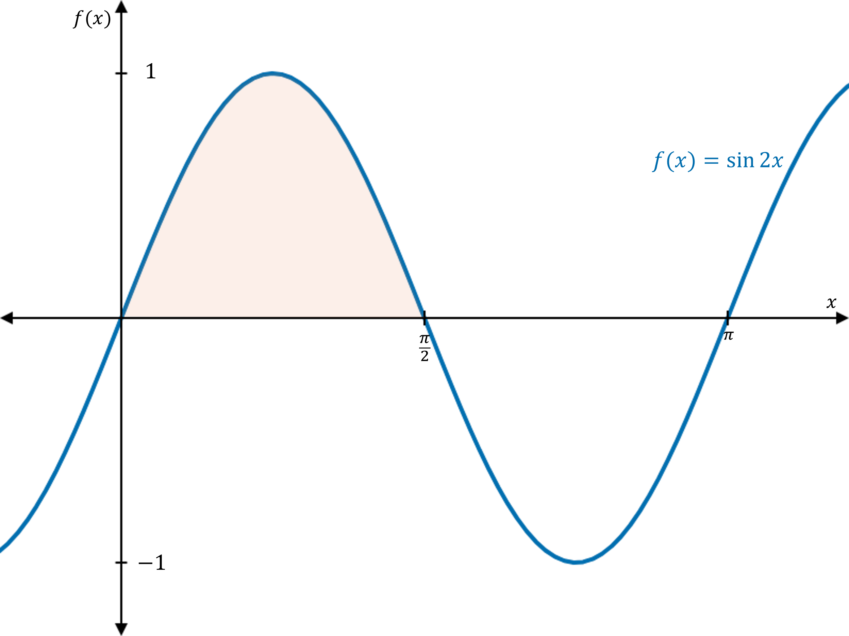
The area bound between the curve \(f(x) = \sin(2x)\) and the \(x\)-axis for \(x \in [0,\frac{\pi}{2}]\) can be found:
\[\displaystyle \begin{align} \int_{0}^{{\frac{\pi}{2}}}\sin{\left(2x\right)}dx &=\left[-\frac{1}{2}\cos{\left(2x\right)}\right]_0^{{\frac{\pi}{2}}}\\ &=-\frac{1}{2}\left[\cos{\left(\pi\right)}-\cos{(0)}\right]_0^{\frac{\pi}{2}}\\ &=-\frac{1}{2}\left(-1-1\right) \\ &=2 \end{align}\]