Basics of graphs and networks
Graphs and networks are powerful tools for representing connections or relationships between objects or people. They belong to a branch of mathematics called graph theory which is quite distinct from other types of mathematics that may have been previously encountered. Therefore, to effectively apply these concepts, it is essential to understand some of the basic definitions and how graphs and networks are diagrammatically.
Use this page to revise the following concepts within basics of graphs and networks:
Graph Definitions
A solid understanding of the basic definitions is essential for understanding graphs, their practical applications and the key differences that distinguish them from networks.
Basic Terminology
A graph is a diagram that shows connections between objects.
- Vertices are labelled dots on the graph which represent objects.
- Edges are lines on the graph between an object or objects which represent the connections. Edges must connect from one vertex to another.
- Loops are a special type of edge that connects a vertex to itself.

The degree of a vertex describes the number of edges that connect to it. They can be classified as:
- Even: having an even number of edges connected
- Odd: having an odd number of edges connected
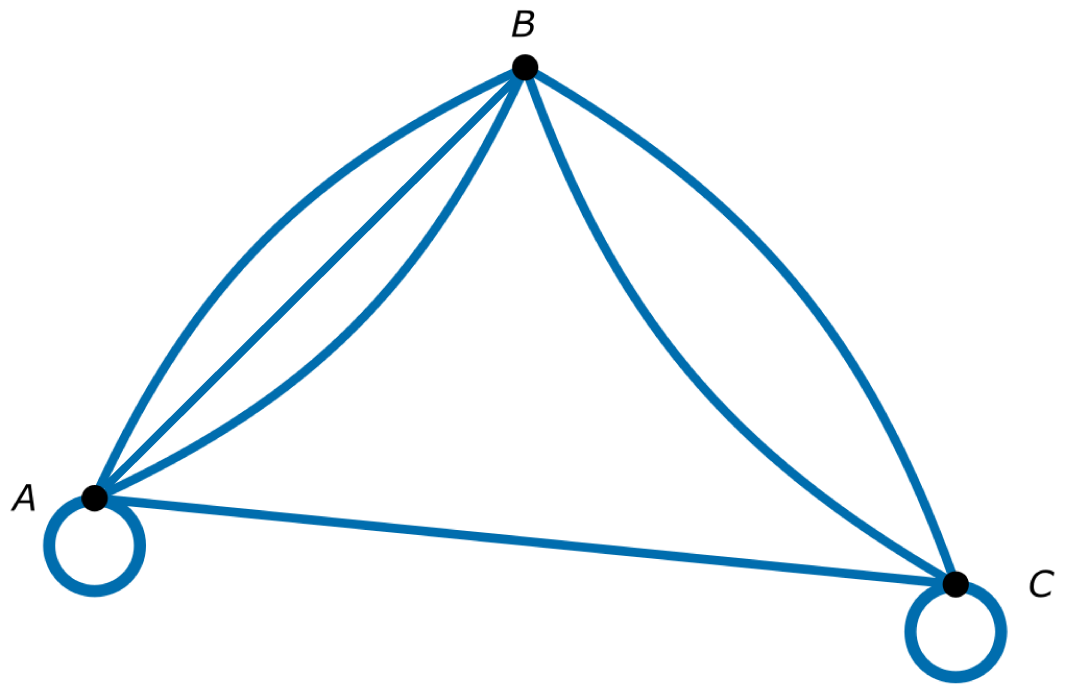
For example, in the image above, the degree of vertex B is 4 \((\deg(B)=4)\).
This means that there are four edges that connect to vertex B.
A loop is counted as two degrees since both the ends of the edge connect to the same vertex. For example, in the image above, the degree of vertex D is 3 \((\deg(D)=3)\). This means there are “three” edges connected to it – the loop and the edge from B to D.
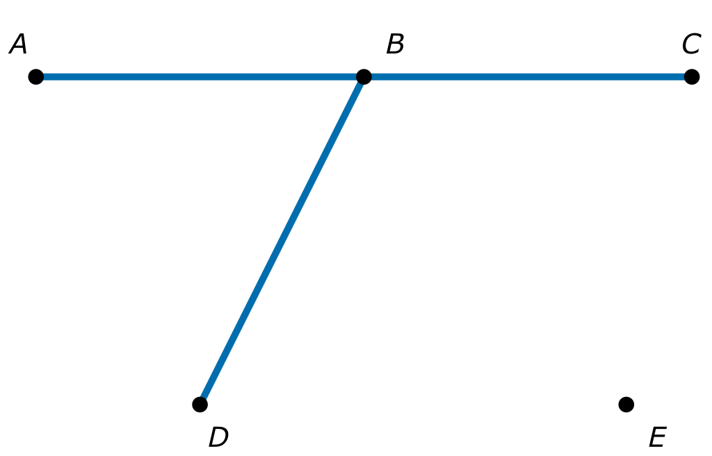
Isolated vertices are vertices that are not connected to any other vertex. For example, in the image above, vertex E is an isolated vertex.
Vertices can have multiple edges between them. In the above example, there are two edges from B to C.
 Check your understanding
View
Check your understanding
View

Graph Descriptions
There are different ways to describe the overall graph:


Check your understanding
View
Euler’s Rule
Faces are areas that are enclosed by edges in a planar graph. This includes both within and outside the areas.

The image above illustrates what is meant by enclosed by edges (highlighted). The number of faces includes the inside regions (faces 1 & 2), as well as the overall outside (face 3).
NoteAreas enclosed by just edges, and not vertices, are not considered faces.
|

Euler’s rule describes the relationship between vertices, edges and faces in a planar graph:
Where:
Worked Example
If a graph has 5 vertices, 6 edges, and 3 faces. Determine if it is planar.
\[5-6+3=-1+3=2\]
As this satisfies Euler’s rule, the graph is planar.
Check your understanding
View
Directed Graphs and Networks
Directed graphs are graphs where edges have a direction represented by arrows. These arrows indicate a one-way connection between two vertices, which is important for modelling applications such as flow or task dependencies.
Networks are graphs with weighted edges, where numerical values on edges specific quantities such as distance, time, or capacity. These can be either directed or undirected, and invaluable for applications involving measurable connections.
Representation of Graphs
Graphs can be represented as diagrams with the features and structures described, but also as adjacency matrices. Adjacency matrices are a way to represent the connections between the vertices on a graph numerically. Adjacency matrices are square matrices where the corresponding rows and columns represent each of the vertices. The elements (values entered) of the matrix represent the number of edges between the respective vertices.
NoteImportant: Loops are only considered 1 edge in an adjacency matrix, although considered as 2 degrees when determining the degree of a vertex. |
If there are vertices \(A, B\), and \(C\) in a graph, the following \(3\times 3\) matrix can be constructed:
\(\space\space\space\space\space\space\space A\space\space\space B\space\space\space C\space\space\space\)
\(\begin{align}& A\\& B\\& C\end{align}\) \(\left[\begin{align}& \Box\space\space\space \Box\space\space\space \Box\\& \Box\space\space\space \Box\space\space\space \Box\\& \Box\space\space\space \Box\space\space\space \Box\end{align}\right]\)
For undirected graphs, these matrices are also symmetrical.
The main diagonal represents the connections between the vertex and itself – loops.
Worked Example
Construct an adjacency matrix to represent the following graph.
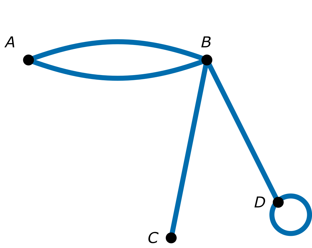
The graph has four vertices, therefore a \(4\times 4\) adjacency matrix is required to describe the connections.
\(\space\space\space\space A\space\space\space B\space\space\space C\space\space\space D\)
\(\begin{align}& A\\& B\\& C\\& D\end{align}\) \(\left[\begin{align}& \Box\space\space\space \Box\space\space\space \Box\space\space\space \Box\\& \Box\space\space\space \Box\space\space\space \Box\space\space\space \Box \\& \Box\space\space\space \Box\space\space\space \Box\space\space\space \Box \\& \Box\space\space\space \Box\space\space\space \Box\space\space\space \Box\end{align}\right]\)
Identify the edges
\(A\) to \(B:2\)
\(B\) to \(C:1\)
\(B\) to \(D:1\)
\(D\) to \(D:1\)
Fill in the matrix – recall that an undirected graph produces a symmetric matrix.
\(\space\space\space\space A\space\space\space B\space\space\space C\space\space\space D\)
\(\begin{align}& A\\& B\\& C\\& D\end{align}\) \(\left[\begin{align}& 0\space\space\space \textcolor{red}{2}\space\space\space 0\space\space\space 0\\& 2\space\space\space 0\space\space\space \textcolor{red}{1}\space\space\space \textcolor{red}{1} \\& 0\space\space\space 1\space\space\space 0\space\space\space 0\\& 0\space\space\space 1\space\space\space 0\space\space\space 1\end{align}\right]\)
Check your understanding
View
Worked Example
Construct a graph from the following adjacency matrix
\(\space\space\space\space A\space\space B\space\space C\)
\(\begin{align}& A\\& B\\& C\end{align}\) \(\left[\begin{align}& 1\space\space\space 3\space\space\space 1\\& 3\space\space\space 0\space\space\space 2\\& 1\space\space\space 2\space\space\space 1\end{align}\right]\)
The adjacency matrix is \(3\times 3\),which means there are \(3\) vertices.
Identify the edges
\(A\) to \(A:1\)
\(A\) to \(B:3\)
\(A\) to \(C:1\)
\(B\) to \(C:2\)
\(C\) to \(C:1\)
Draw the graph